Variance homogeneity in two or more groups

TODO

• link to variance

Install required packages

car, coin, beeswarm

wants <- c("car", "coin", "beeswarm")
has   <- wants %in% rownames(installed.packages())
if(any(!has)) install.packages(wants[!has])

Compare two groups

Boxplot with added beeswarm plot

set.seed(123)
P     <- 2
Nj    <- c(50, 40)
DV1   <- rnorm(Nj[1], mean=100, sd=15)
DV2   <- rnorm(Nj[2], mean=100, sd=13)
varDf <- data.frame(DV=c(DV1, DV2),
                    IV=factor(rep(1:P, Nj)))

library(beeswarm)
boxplot(DV ~ IV, data=varDf)
beeswarm(DV ~ IV, data=varDf, add=TRUE, pch=16, col="#00000077")

\(F\)-test for variance ratio in two groups

var.test(DV1, DV2)

var.test(DV ~ IV, data=varDf)

    F test to compare two variances

data:  DV by IV
F = 1.5437, num df = 49, denom df = 39, p-value = 0.1632
alternative hypothesis: true ratio of variances is not equal to 1
95 percent confidence interval:
 0.8361247 2.7913772
sample estimates:
ratio of variances 
          1.543726 

Mood-test for two groups (nonparametric)

mood.test(DV ~ IV, alternative="greater", data=varDf)

    Mood two-sample test of scale

data:  DV by IV
Z = 1.8065, p-value = 0.03542
alternative hypothesis: greater

Ansari-Bradley-test for two groups (nonparametric)

ansari.test(DV ~ IV, alternative="greater", exact=FALSE, data=varDf)

    Ansari-Bradley test

data:  DV by IV
AB = 1025, p-value = 0.02116
alternative hypothesis: true ratio of scales is greater than 1

library(coin)
ansari_test(DV ~ IV, alternative="greater", distribution="exact", data=varDf)

    Exact Two-Sample Ansari-Bradley Test

data:  DV by IV (1, 2)
Z = -2.0304, p-value = 0.02138
alternative hypothesis: true ratio of scales is greater than 1

Compare more than two groups

Boxplot with added beeswarm plot

Nj    <- c(22, 18, 20)
N     <- sum(Nj)
P     <- length(Nj)
levDf <- data.frame(DV=sample(0:100, N, replace=TRUE),
                    IV=factor(rep(1:P, Nj)))

library(beeswarm)
boxplot(DV ~ IV, data=levDf)
beeswarm(DV ~ IV, data=levDf, add=TRUE, pch=16, col="#00000077")

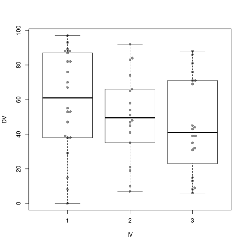
Levene-test

library(car)
leveneTest(DV ~ IV, center=median, data=levDf)

Levene's Test for Homogeneity of Variance (center = median)
      Df F value Pr(>F)
group  2  0.5531 0.5782
      57               

leveneTest(DV ~ IV, center=mean, data=levDf)

Levene's Test for Homogeneity of Variance (center = mean)
      Df F value Pr(>F)
group  2  0.5865 0.5596
      57               

Fligner-Killeen-test

fligner.test(DV ~ IV, data=levDf)

    Fligner-Killeen test of homogeneity of variances

data:  DV by IV
Fligner-Killeen:med chi-squared = 0.68727, df = 2, p-value = 0.7092

library(coin)
fligner_test(DV ~ IV, distribution=approximate(nresample=9999), data=levDf)

    Approximative K-Sample Fligner-Killeen Test

data:  DV by IV (1, 2, 3)
chi-squared = 0.68727, p-value = 0.7067

Detach (automatically) loaded packages (if possible)

try(detach(package:car))
try(detach(package:carData))
try(detach(package:coin))
try(detach(package:survival))
try(detach(package:beeswarm))

Get the article source from GitHub

R markdown - markdown - R code - all posts