Survival analysis: Kaplan-Meier
TODO
- link to survivalCoxPH, survivalParametric
Install required packages
wants <- c("survival")
has   <- wants %in% rownames(installed.packages())
if(any(!has)) install.packages(wants[!has])
Simulated right-censored event times with Weibull distribution
Simulated survival time \(T\) influenced by time independent covariates \(X_{j}\) with effect parameters \(\beta_{j}\) under assumption of proportional hazards, stratified by sex.
\(T = (-\ln(U) \, b \, e^{-\bf{X} \bf{\beta}})^{\frac{1}{a}}\), where \(U \sim \mathcal{U}(0, 1)\), \(a\) is the Weibull shape parameter and \(b\) is the Weibull scale parameter.
set.seed(123)
N      <- 180                  # number of observations
P      <- 3                    # number of groups
sex    <- factor(sample(c("f", "m"), N, replace=TRUE))  # stratification factor
X      <- rnorm(N, 0, 1)       # continuous covariate
IV     <- factor(rep(LETTERS[1:P], each=N/P))  # factor covariate
IVeff  <- c(0, -1, 1.5)        # effects of factor levels (1 -> reference level)
Xbeta  <- 0.7*X + IVeff[unclass(IV)] + rnorm(N, 0, 2)
weibA  <- 1.5                  # Weibull shape parameter
weibB  <- 100                  # Weibull scale parameter
U      <- runif(N, 0, 1)       # uniformly distributed RV
eventT <- ceiling((-log(U)*weibB*exp(-Xbeta))^(1/weibA))   # simulated event time

# censoring due to study end after 120 days
obsLen <- 120                  # length of observation time
censT  <- rep(obsLen, N)       # censoring time = end of study
obsT   <- pmin(eventT, censT)  # observed censored event times
status <- eventT <= censT      # has event occured?
dfSurv <- data.frame(obsT, status, sex, X, IV)          # data frame
Survival data in counting process (start-stop) notation.
library(survival)
dfSurvCP <- survSplit(dfSurv, cut=seq(30, 90, by=30), end="obsT",
                      event="status", start="start", id="ID", zero=0)
Plot simulated data
plot(ecdf(eventT), xlim=c(0, 200), main="Cumulative survival distribution",
     xlab="t", ylab="F(t)", cex.lab=1.4)
abline(v=obsLen, col="blue", lwd=2)
text(obsLen-5, 0.2, adj=1, labels="end of study", cex=1.4)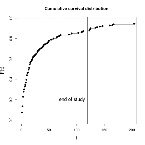
Kaplan-Meier-Analysis
Estimate survival-function
Survival function \(S(t) = 1-F(t)\), hazard function
\[ \begin{equation*} \lambda(t) = \lim_{\Delta_{t} \to 0^{+}} \frac{P(t \leq T < t + \Delta_{t} \, | \, T \geq t)}{\Delta_{t}} = \frac{P(t \leq T < t + \Delta_{t}) / \Delta_{t}}{P(T > t)} = \frac{f(t)}{S(t)}, \quad t \geq 0 \end{equation*} \]
library(survival)                # for Surv(), survfit()
## global estimate
KM0 <- survfit(Surv(obsT, status) ~ 1,  type="kaplan-meier", conf.type="log", data=dfSurv)

## separate estimate for all strata
(KM <- survfit(Surv(obsT, status) ~ IV, type="kaplan-meier", conf.type="log", data=dfSurv))
Call: survfit(formula = Surv(obsT, status) ~ IV, data = dfSurv, type = "kaplan-meier",
conf.type = "log")
records n.max n.start events median 0.95LCL 0.95UCL
IV=A 60 60 60 53 13.0 8 29
IV=B 60 60 60 46 35.0 20 58
IV=C 60 60 60 58 9.5 4 13Arbitrary quantiles for estimated survival function.
quantile(KM0, probs=c(0.25, 0.5, 0.75), conf.int=FALSE) 25 50 75
4.0 14.0 46.5 50-day and 100-day survival including point-wise confidence interval.
summary(KM0, times=c(50, 100))Call: survfit(formula = Surv(obsT, status) ~ 1, data = dfSurv, type = "kaplan-meier",
conf.type = "log")
time n.risk n.event survival std.err lower 95% CI upper 95% CI
50 42 140 0.222 0.0310 0.169 0.292
100 27 13 0.150 0.0266 0.106 0.212All estimated values for survival function including point-wise confidence interval.
summary(KM0)
# not shown
Plot estimated survival function
Global estimate including pointwise confidence intervals.
plot(KM0, main=expression(paste("Kaplan-Meier-estimate ", hat(S)(t), " with CI")),
     xlab="t", ylab="Survival", lwd=2)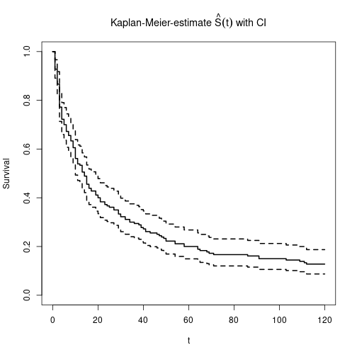
Separate estimates for levels of factor IV
plot(KM, main=expression(paste("Kaplan-Meier-estimate ", hat(S)[g](t), " for groups g")),
     xlab="t", ylab="Survival", lwd=2, col=1:3)
legend(x="bottomright", col=1:3, lwd=2, legend=LETTERS[1:3])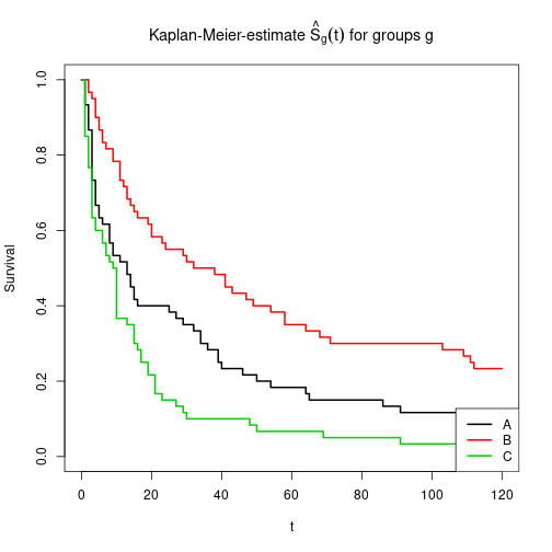
Plot cumulative incidence function
Separate estimates for levels of factor IV
plot(KM, main=expression(paste("KM cumulative incidence 1-", hat(S)[g](t), " for groups g")),
     fun=function(x) { 1- x },
     xlab="t", ylab="Cumulative incidence", lwd=2, col=1:3)
legend(x="topright", col=1:3, lwd=2, legend=LETTERS[1:3])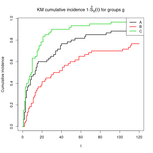
Plot cumulative hazard
\(\hat{\Lambda}(t)\)
plot(KM0, main=expression(paste("Kaplan-Meier-estimate ", hat(Lambda)(t))),
     xlab="t", ylab="cumulative hazard", fun="cumhaz", lwd=2)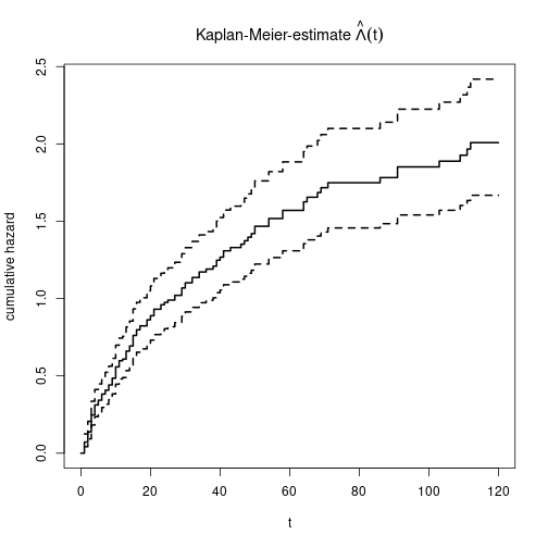
Log-rank-test for equal survival-functions
Global test
library(survival)
survdiff(Surv(obsT, status) ~ IV, data=dfSurv)
Call:
survdiff(formula = Surv(obsT, status) ~ IV, data = dfSurv)
N Observed Expected (O-E)^2/E (O-E)^2/V
IV=A 60 53 49.9 0.196 0.301
IV=B 60 46 71.7 9.220 18.251
IV=C 60 58 35.4 14.402 20.264
Chisq= 26.1 on 2 degrees of freedom, p= 2.16e-06 Stratified for factor sex
library(survival)
survdiff(Surv(obsT, status) ~ IV + strata(sex), data=dfSurv)
Call:
survdiff(formula = Surv(obsT, status) ~ IV + strata(sex), data = dfSurv)
N Observed Expected (O-E)^2/E (O-E)^2/V
IV=A 60 53 49.7 0.225 0.345
IV=B 60 46 71.9 9.311 18.516
IV=C 60 58 35.5 14.302 20.127
Chisq= 26.1 on 2 degrees of freedom, p= 2.12e-06 Detach (automatically) loaded packages (if possible)
try(detach(package:survival))
try(detach(package:splines))
Get the article source from GitHub
R markdown - markdown - R code - all posts