Visualize univariate and bivariate distributions
- TODO
- Install required packages
- Histograms
- Stem and leaf plot
- Boxplot
- Dotchart
- Stripchart
- QQ-plot
- Empirical cumulative distribution function
- Joint distribution of two variables in separate groups
- Joint distribution of two variables with many observations
- Detach (automatically) loaded packages (if possible)
- Get the article source from GitHub
TODO
- link to diagCategorical, diagScatter, diagMultivariate, diagAddElements, diagBounding
- new R 2.15.1+
qqplot()optionsdistributionandprobs
Install required packages
wants <- c("car", "hexbin")
has   <- wants %in% rownames(installed.packages())
if(any(!has)) install.packages(wants[!has])
Histograms
Histogram with absolute class frequencies
set.seed(123)
x <- rnorm(200, 175, 10)
hist(x, xlab="x", ylab="N", breaks="FD")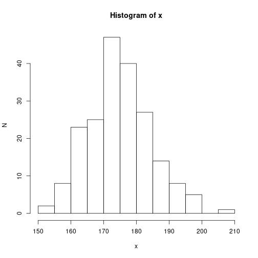
Add individual values and normal probability density function
hist(x, freq=FALSE, xlab="x", ylab="relative frequency",
     breaks="FD", main="Histogram und normal PDF")
rug(jitter(x))
curve(dnorm(x, mean(x), sd(x)), lwd=2, col="blue", add=TRUE)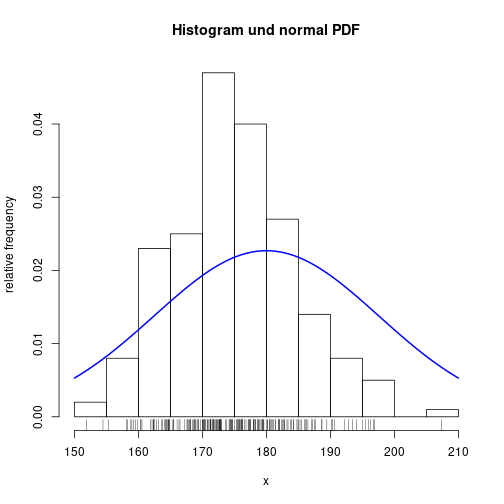
Add estimated probability density function
hist(x, freq=FALSE, xlab="x", breaks="FD",
     main="Histogram and density estimate")
lines(density(x), lwd=2, col="blue")
rug(jitter(x))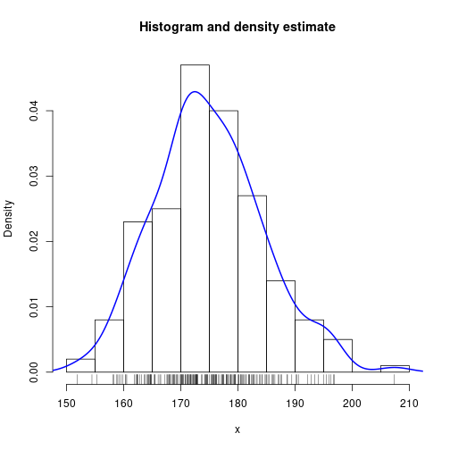
To compare the histograms from two groups, see histbackback() from package Hmisc.
Stem and leaf plot
y <- rnorm(100, mean=175, sd=7)
stem(y)
  The decimal point is 1 digit(s) to the right of the |

  15 | 669
  16 | 134
  16 | 5566777789
  17 | 0011112222233333334444444
  17 | 5555566666677777788888888999
  18 | 0000000001111233334444
  18 | 55667779
  19 | 2
Boxplot
Nj <- 40
P  <- 3
DV <- rnorm(P*Nj, mean=100, sd=15)
IV <- gl(P, Nj, labels=c("Control", "Group A", "Group B"))boxplot(DV ~ IV, ylab="Score", col=c("red", "blue", "green"),
main="Boxplot of scores in 3 groups")
stripchart(DV ~ IV, pch=16, col="darkgray", vert=TRUE, add=TRUE)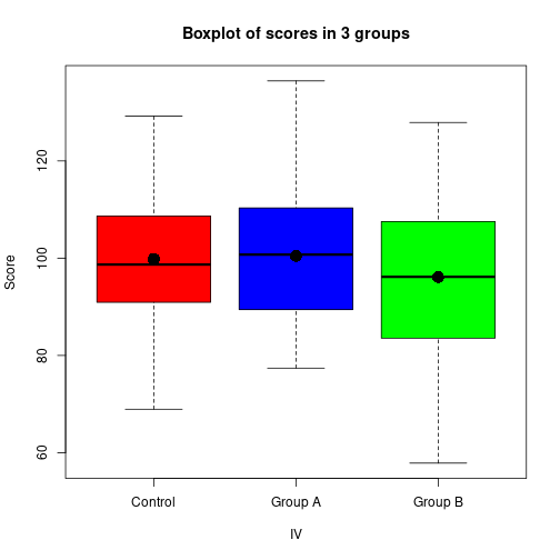
xC <- DV[IV == "Control"]
xA <- DV[IV == "Group A"]
boxplot(xC, xA)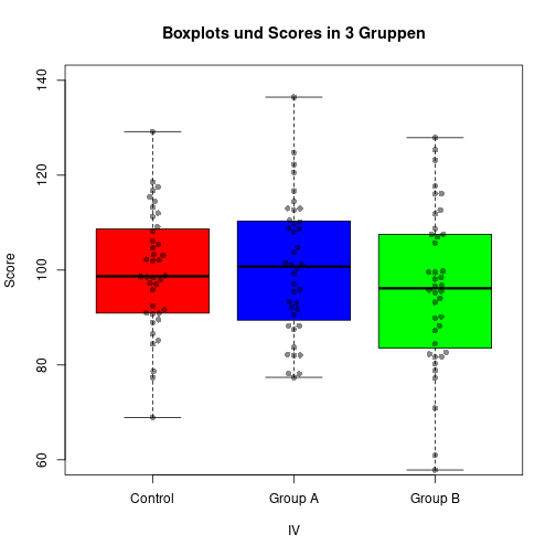
Dotchart
Nj  <- 5
DV1 <- rnorm(Nj, 20, 2)
DV2 <- rnorm(Nj, 25, 2)
DV  <- c(DV1, DV2)
IV  <- gl(2, Nj)
Mj <- tapply(DV, IV, FUN=mean)dotchart(DV, gdata=Mj, pch=16, color=rep(c("red", "blue"), each=Nj),
gcolor="black", labels=rep(LETTERS[1:Nj], 2), groups=IV,
xlab="AV", ylab="group",
main="individual results and means from 2 groups")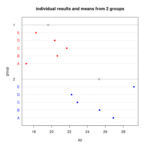
Stripchart
Nj   <- 25
P    <- 4
dice <- sample(1:6, P*Nj, replace=TRUE)
IV <- gl(P, Nj)stripchart(dice ~ IV, xlab="Result", ylab="group", pch=1, col="blue",
main="Dice results: 4 groups", sub="jitter-method", method="jitter")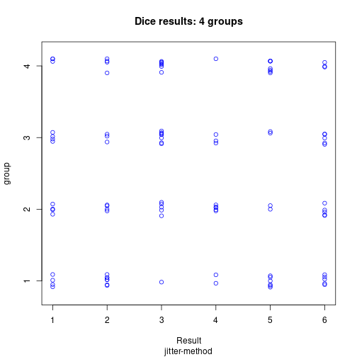
stripchart(dice ~ IV, xlab="Result", ylab="group", pch=16, col="red",
           main="Dice results: 4 groups", sub="stack-method", method="stack")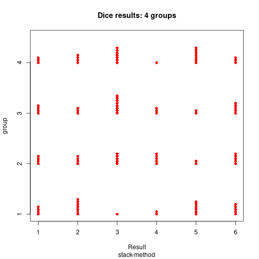
QQ-plot
DV1 <- rnorm(200)
DV2 <- rf(200, df1=3, df2=15)
qqplot(DV1, DV2, xlab="quantile N(0, 1)", ylab="quantile F(3, 15)",
       main="Comparison of quantiles from N(0, 1) and F(3, 15)")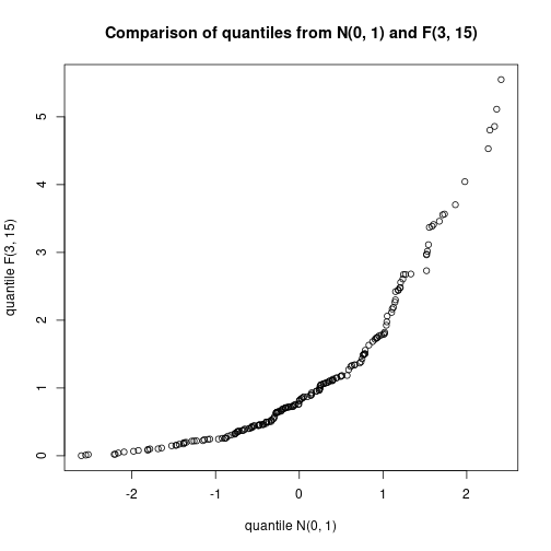
height <- rnorm(100, mean=175, sd=7)
qqnorm(height)
qqline(height, col="red", lwd=2)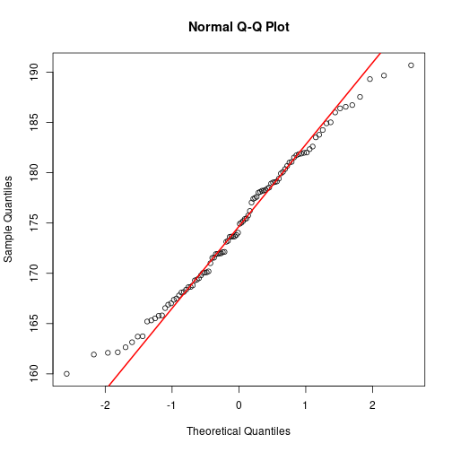
Empirical cumulative distribution function
vec <- round(rnorm(10), 1)
Fn  <- ecdf(vec)
plot(Fn, main="Empirical cumulative distribution function")
curve(pnorm, add=TRUE, col="gray", lwd=2)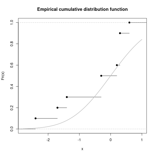
Joint distribution of two variables in separate groups
Simulate data
N  <- 200
P  <- 2
x  <- rnorm(N, 100, 15)
y  <- 0.5*x + rnorm(N, 0, 10)
IV <- gl(P, N/P, labels=LETTERS[1:P])
Identify group membership by plot symbol and color
plot(x, y, pch=c(4, 16)[unclass(IV)], lwd=2,
     col=c("black", "blue")[unclass(IV)],
     main="Joint distribution per group")
legend(x="topleft", legend=c("group A", "group B"),
       pch=c(4, 16), col=c("black", "blue"))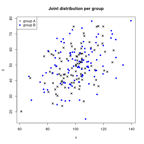
Add distribution ellipse
Pooled groups
library(car)
dataEllipse(x, y, xlab="x", ylab="y", asp=1, levels=0.5, lwd=2, center.pch=16,
            col="blue", main="Joint distribution of two variables")
legend(x="bottomright", legend=c("Data", "centroid", "distribution ellipse"),
       pch=c(1, 16, NA), lty=c(NA, NA, 1), col=c("black", "blue", "blue"))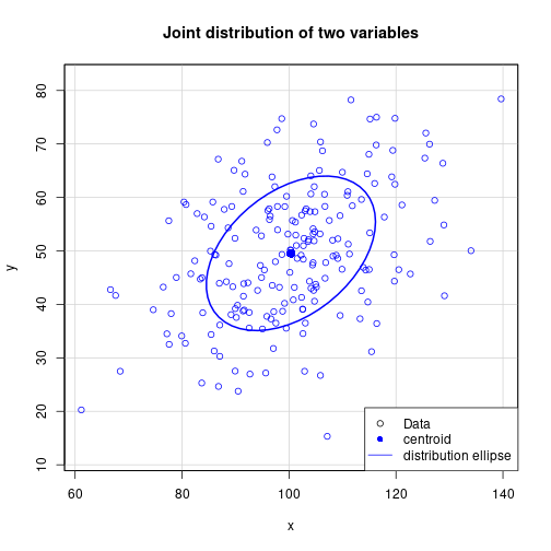
Joint distribution of two variables with many observations
Using transparency
N  <- 5000
xx <- rnorm(N, 100, 15)
yy <- 0.4*xx + rnorm(N, 0, 10)
plot(xx, yy, pch=16, col=rgb(0, 0, 1, 0.3))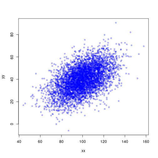
Smooth scatter plot
Based on a 2-D kernel density estimate
smoothScatter(xx, yy, bandwidth=4)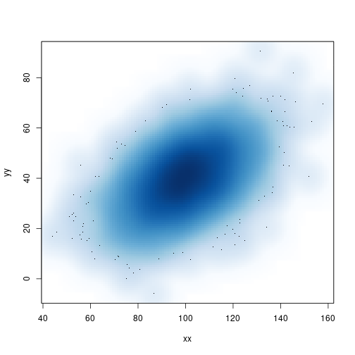
Hexagonal 2-D binning
library(hexbin)
res <- hexbin(xx, yy, xbins=20)
plot(res)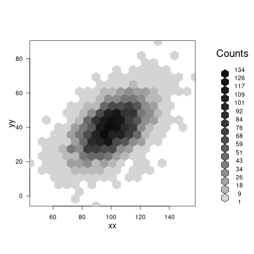
summary(res)'hexbin' object from call: hexbin(x = xx, y = yy, xbins = 20)
n = 5000 points in nc = 214 hexagon cells in grid dimensions 26 by 21
cell count xcm ycm
Min. : 9.0 Min. : 1.00 Min. : 44.83 Min. :-5.868
1st Qu.:156.2 1st Qu.: 2.00 1st Qu.: 81.19 1st Qu.:23.484
Median :240.5 Median : 8.00 Median :101.46 Median :40.020
Mean :241.7 Mean : 23.36 Mean :101.18 Mean :40.089
3rd Qu.:324.8 3rd Qu.: 31.00 3rd Qu.:120.83 3rd Qu.:56.395
Max. :499.0 Max. :133.00 Max. :157.78 Max. :90.498 Detach (automatically) loaded packages (if possible)
try(detach(package:car))
try(detach(package:hexbin))
Get the article source from GitHub
R markdown - markdown - R code - all posts