Survival analysis: Cox proportional hazards model
- TODO
- Install required packages
- Simulated right-censored event times with Weibull distribution
- Fit the Cox proportional hazards model
- Assess model fit
- Estimate survival-function und cumulative baseline hazard
- Model diagnostics
- Predicted hazard ratios
- Further resources
- Detach (automatically) loaded packages (if possible)
- Get the article source from GitHub
TODO
- link to survivalKM, survivalParametric
Install required packages
wants <- c("survival")
has   <- wants %in% rownames(installed.packages())
if(any(!has)) install.packages(wants[!has])
Simulated right-censored event times with Weibull distribution
Time independent covariates with proportional hazards
\(T = (-\ln(U) \, b \, e^{-\bf{X} \bf{\beta}})^{\frac{1}{a}}\), where \(U \sim \mathcal{U}(0, 1)\)
set.seed(123)
N      <- 180
P      <- 3
sex    <- factor(sample(c("f", "m"), N, replace=TRUE))
X      <- rnorm(N, 0, 1)
IV     <- factor(rep(LETTERS[1:P], each=N/P))
IVeff  <- c(0, -1, 1.5)
Xbeta  <- 0.7*X + IVeff[unclass(IV)] + rnorm(N, 0, 2)
weibA  <- 1.5
weibB  <- 100
U      <- runif(N, 0, 1)
eventT <- ceiling((-log(U)*weibB*exp(-Xbeta))^(1/weibA))
obsLen <- 120
censT  <- rep(obsLen, N)
obsT   <- pmin(eventT, censT)
status <- eventT <= censT
dfSurv <- data.frame(obsT, status, sex, X, IV)
Survival data in counting process (start-stop) notation.
library(survival)
dfSurvCP <- survSplit(dfSurv, cut=seq(30, 90, by=30), end="obsT",
                      event="status", start="start", id="ID", zero=0)
Fit the Cox proportional hazards model
Assumptions
\[ \begin{equation*} \begin{array}{rclcl} \ln \lambda(t) &=& \ln \lambda_{0}(t) + \beta_{1} X_{1} + \dots + \beta_{p} X_{p} &=& \ln \lambda_{0}(t) + \bf{X} \bf{\beta}\\ \lambda(t) &=& \lambda_{0}(t) \, e^{\beta_{1} X_{1} + \dots + \beta_{p} X_{p}} &=& \lambda_{0}(t) \, e^{\bf{X} \bf{\beta}}\\ S(t) &=& S_{0}(t)^{\exp(\bf{X} \bf{\beta})} &=& \exp\left(-\Lambda_{0}(t) \, e^{\bf{X} \bf{\beta}}\right)\\ \Lambda(t) &=& \Lambda_{0}(t) \, e^{\bf{X} \bf{\beta}} & & \end{array} \end{equation*} \]
library(survival)
(fitCPH <- coxph(Surv(obsT, status) ~ X + IV, data=dfSurv))
Call:
coxph(formula = Surv(obsT, status) ~ X + IV, data = dfSurv)
coef exp(coef) se(coef) z p
X 0.493 1.637 0.0937 5.26 1.4e-07
IVB -0.822 0.439 0.2108 -3.90 9.6e-05
IVC 0.377 1.457 0.1934 1.95 5.1e-02
Likelihood ratio test=51.6 on 3 df, p=3.62e-11 n= 180, number of events= 157 Use counting process data format.
coxph(Surv(start, obsT, status) ~ X + IV, data=dfSurvCP)
summary(fitCPH)
# not shown
Assess model fit
AIC
library(survival)
extractAIC(fitCPH)
[1] 3.000 1367.667McFadden, Cox & Snell and Nagelkerke pseudo \(R^{2}\)
Log-likelihoods for full model and 0-model without predictors X1, X2
LLf <- fitCPH$loglik[2]
LL0 <- fitCPH$loglik[1]
McFadden pseudo-\(R^2\)
as.vector(1 - (LLf / LL0))[1] 0.0365218Cox & Snell
as.vector(1 - exp((2/N) * (LL0 - LLf)))[1] 0.2493033Nagelkerke
as.vector((1 - exp((2/N) * (LL0 - LLf))) / (1 - exp(LL0)^(2/N)))[1] 0.2494003Model comparisons
Restricted model without factor IV
library(survival)
fitCPH1 <- coxph(Surv(obsT, status) ~ X, data=dfSurv)
anova(fitCPH1, fitCPH)          # model comparison
Analysis of Deviance Table
Cox model: response is Surv(obsT, status)
Model 1: ~ X
Model 2: ~ X + IV
loglik Chisq Df P(>|Chi|)
1 -698.77
2 -680.83 35.867 2 1.628e-08 ***
---
Signif. codes: 0 '***' 0.001 '**' 0.01 '*' 0.05 '.' 0.1 ' ' 1Estimate survival-function und cumulative baseline hazard
Survival function
For average pseudo-observation with covariate values equal to the sample means. For factors: means of dummy-coded indicator variables.
library(survival)                # for survfit()
(CPH <- survfit(fitCPH))
Call: survfit(formula = fitCPH)
records n.max n.start events median 0.95LCL 0.95UCL
180 180 180 157 14 11 19 quantile(CPH, probs=c(0.25, 0.5, 0.75), conf.int=FALSE)25 50 75
4 14 39 More meaningful: Estimated survival function for new specific data
dfNew  <- data.frame(sex=factor(c("f", "f"), levels=levels(dfSurv$sex)),
                       X=c(-2, -2),
                      IV=factor(c("A", "C"), levels=levels(dfSurv$IV)))

library(survival)
CPHnew <- survfit(fitCPH, newdata=dfNew)

par(mar=c(5, 4.5, 4, 2)+0.1, cex.lab=1.4, cex.main=1.4)
plot(CPH, main=expression(paste("Cox PH-estimate ", hat(S)(t), " with CI")),
     xlab="t", ylab="Survival", lwd=2)
lines(CPHnew$time, CPHnew$surv[ , 1], lwd=2, col="blue")
lines(CPHnew$time, CPHnew$surv[ , 2], lwd=2, col="red")
legend(x="topright", lwd=2, col=c("black", "blue", "red"),
       legend=c("pseudo-observation", "sex=f, X=-2, IV=A", "sex=f, X=-2, IV=C"))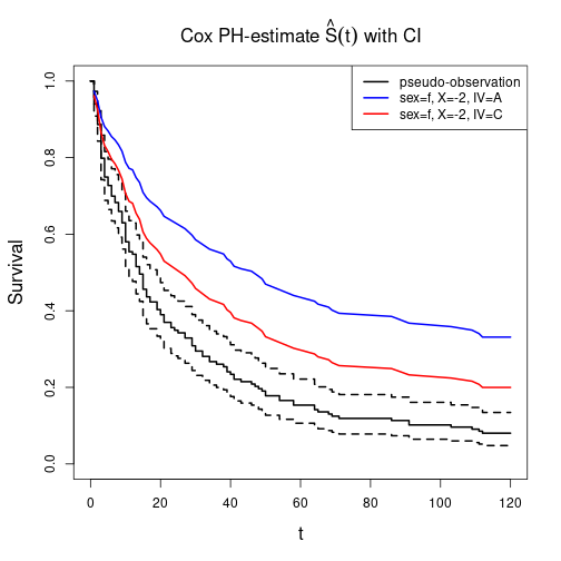
Cumulative baseline hazard
library(survival)                # for basehaz()
expCoef  <- exp(coef(fitCPH))
Lambda0A <- basehaz(fitCPH, centered=FALSE)
Lambda0B <- expCoef[2]*Lambda0A$hazard
Lambda0C <- expCoef[3]*Lambda0A$hazard
plot(hazard ~ time, main=expression(paste("Cox PH-estimate ", hat(Lambda)[g](t), " per group")),
     type="s", ylim=c(0, 5), xlab="t", ylab="cumulative hazard", lwd=2, data=Lambda0A)
lines(Lambda0A$time, Lambda0B, lwd=2, col="red")
lines(Lambda0A$time, Lambda0C, lwd=2, col="green")
legend(x="bottomright", lwd=2, col=1:3, legend=LETTERS[1:3])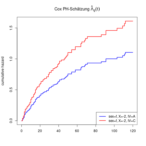
Model diagnostics
Proportional hazards assumption
log-log plot for categorized predictor X.
library(survival)                # for survfit()
dfSurv <- transform(dfSurv, Xcut=cut(X, breaks=c(-Inf, median(X), Inf),
                                        labels=c("lo", "hi")))
KMiv   <- survfit(Surv(obsT, status) ~ IV,   type="kaplan-meier", data=dfSurv)
KMxcut <- survfit(Surv(obsT, status) ~ Xcut, type="kaplan-meier", data=dfSurv)

plot(KMiv, fun="cloglog", main="cloglog-Plot for IV1", xlab="ln t",
     ylab=expression(ln(-ln(hat(S)[g](t)))), col=c("black", "blue", "red"), lty=1:3)

legend(x="topleft", col=c("black", "blue", "red"), lwd=2, lty=1:3, legend=LETTERS[1:3])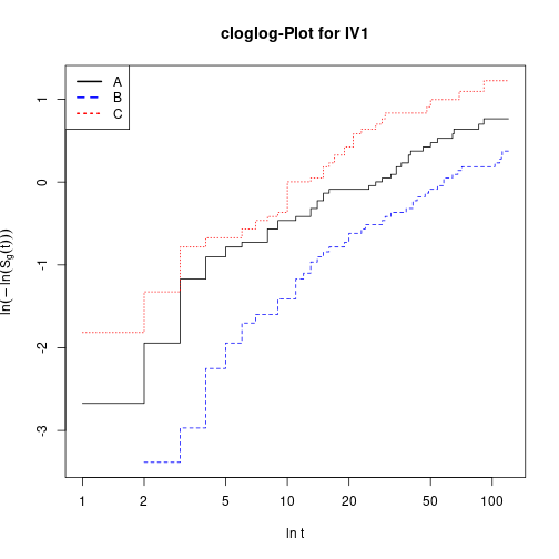
plot(KMxcut, fun="cloglog", main="cloglog-Plot for Xcut", xlab="ln t",
     ylab=expression(ln(-ln(hat(S)[g](t)))), col=c("black", "blue"), lty=1:2)

legend(x="topleft", col=c("black", "blue"), lwd=2, lty=1:2, legend=c("lo", "hi"))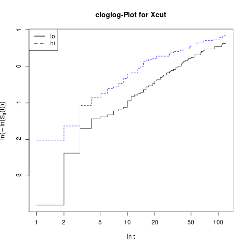
Test based on scaled Schoenfeld-residuals
library(survival)                      # for cox.zph()
(czph <- cox.zph(fitCPH))
rho chisq p
X -0.1039 2.073 0.1500
IVB 0.1559 4.006 0.0453
IVC 0.0406 0.265 0.6069
GLOBAL NA 5.053 0.1680Plot scaled Schoenfeld-residuals against covariates
par(mfrow=c(2, 2), cex.main=1.4, cex.lab=1.4)
plot(czph)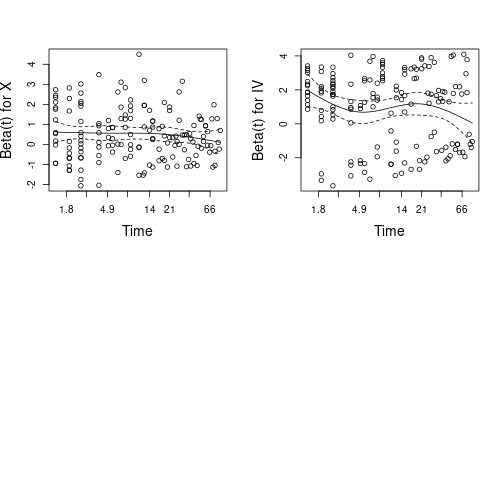
Influential observations
dfbetas <- residuals(fitCPH, type="dfbetas")

par(mfrow=c(2, 2), cex.main=1.4, cex.lab=1.4)
plot(dfbetas[ , 1], type="h", main="DfBETAS for X",    ylab="DfBETAS", lwd=2)
plot(dfbetas[ , 2], type="h", main="DfBETAS for IV-B", ylab="DfBETAS", lwd=2)
plot(dfbetas[ , 3], type="h", main="DfBETAS for IV-C", ylab="DfBETAS", lwd=2)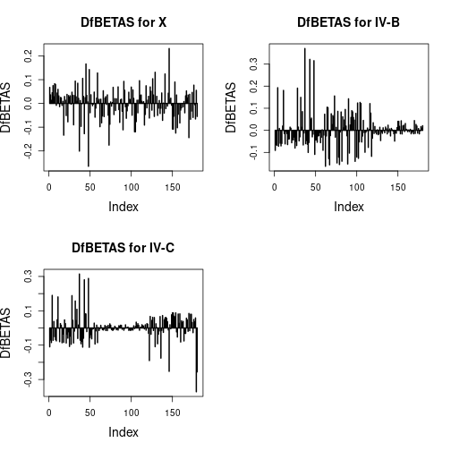
Linearity of log hazard
Plot martingale-residuals against continuous covariate with a nonparametric LOESS-smoother
resMart <- residuals(fitCPH, type="martingale")
plot(dfSurv$X, resMart, main="Martingale-residuals for X",
     xlab="X", ylab="Residuen", pch=20)
lines(loess.smooth(dfSurv$X, resMart), lwd=2, col="blue")
legend(x="bottomleft", col="blue", lwd=2, legend="LOESS fit", cex=1.4)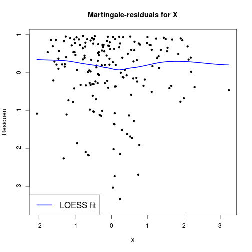
Predicted hazard ratios
With respect to an average pseudo-observation with covariate values equal to the sample means. For factors: means of dummy-coded indicator variables.
library(survival)
predRes <- predict(fitCPH, type="risk")
head(predRes, n=10)
[1] 1.9166403 1.5389801 1.3210722 0.8617067 2.2969713 0.8735328 3.4527637
[8] 2.5002058 1.0455378 0.7079919Estimated global survival function.
library(survival)
Shat1 <- survexp(~ 1, ratetable=fitCPH, data=dfSurv)
with(Shat1, head(data.frame(time, surv), n=4))
time surv
1 1 0.9269729
2 2 0.8643413
3 3 0.7681378
4 4 0.7173365Estimated survival function per group.
library(survival)
Shat2 <- survexp(~ IV, ratetable=fitCPH, data=dfSurv)
with(Shat2, head(data.frame(time, surv), n=4))
time IV.A IV.B IV.C
1 1 0.9265656 0.9633824 0.8909708
2 2 0.8626937 0.9299972 0.8003328
3 3 0.7630677 0.8746553 0.6666905
4 4 0.7097748 0.8431836 0.5990511Further resources
For Cox PH models with Firth’s penalized likelihood, see package coxphf.
Detach (automatically) loaded packages (if possible)
try(detach(package:survival))
try(detach(package:splines))
Get the article source from GitHub
R markdown - markdown - R code - all posts