Root Finding

Case study: Quantile function Hoyt distribution

The cumulative distribution function \(F(x)\) of the Hoyt distribution is given in closed form, but the quantile function \(Q(p)\) is not. \(Q(p)\) = \(F^{-1}(p)\) -> given probability \(p\), find \(x\) such that \(F(x) = p\).

## distribution function
pHoyt <- function(q, qpar, omega) {
    alphaQ <- (sqrt((1 - qpar^4))/(2*qpar)) * sqrt((1 + qpar)/(1 - qpar))
     betaQ <- (sqrt((1 - qpar^4))/(2*qpar)) * sqrt((1 - qpar)/(1 + qpar))

    y <- q / sqrt(omega)
    pchisq((alphaQ*y)^2, df=2, ncp=( betaQ*y)^2) -
    pchisq(( betaQ*y)^2, df=2, ncp=(alphaQ*y)^2)
}

Strictly monotonous function \(f: F() - p\) where the root \(x\) needs to be found such that \(F(x) - p = 0\).

f <- function(x, p, qpar, omega) {
    pHoyt(x, qpar=qpar, omega=omega) - p
}

Implement the quantile function of the Hoyt distribution by doing root finding of \(f\).

qHoyt <- function(p, qpar, omega) {
    uniroot(f, interval=c(0, omega), extendInt="upX",
            p=p, qpar=qpar, omega=omega)$root
}

qHoyt(p=0.7, qpar=0.5, omega=10)

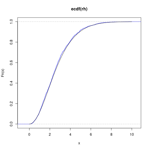
[1] 3.351123

Simulate random deviates from the Hoyt distribution using inverse transform sampling = draw \(p\) from uniform distribution over \([0,1]\) and return \(Q(p)\).

U  <- runif(1000)
rh <- sapply(U, function(x) { qHoyt(p=x, qpar=0.5, omega=10) })

Check that empirical cumulative distribution of random deviates actually follows theoretical cumulative distribution function.

plot(ecdf(rh), col="blue")
curve(pHoyt(x, qpar=0.5, omega=10), from=0, to=10, add=TRUE)

Further resources

• CRAN Task View ‘Numerical Mathematics’

Useful packages

• rootSolve

Get the article source from GitHub

R markdown - markdown - R code - all posts