Survival analysis: Parametric proportional hazards models
TODO
- link to survivalKM, survivalCoxPH
Install required packages
wants <- c("survival")
has   <- wants %in% rownames(installed.packages())
if(any(!has)) install.packages(wants[!has])
Simulated right-censored event times with Weibull distribution
Simulated survival time \(T\) influenced by time independent covariates \(X_{j}\) with effect parameters \(\beta_{j}\) under assumption of proportional hazards, stratified by sex.
\(T = (-\ln(U) \, b \, e^{-\bf{X} \bf{\beta}})^{\frac{1}{a}}\), where \(U \sim \mathcal{U}(0, 1)\), \(a\) is the Weibull shape parameter and \(b\) is the Weibull scale parameter.
set.seed(123)
N      <- 180                  # number of observations
P      <- 3                    # number of groups
sex    <- factor(sample(c("f", "m"), N, replace=TRUE))  # stratification factor
X      <- rnorm(N, 0, 1)       # continuous covariate
IV     <- factor(rep(LETTERS[1:P], each=N/P))  # factor covariate
IVeff  <- c(0, -1, 1.5)        # effects of factor levels (1 -> reference level)
Xbeta  <- 0.7*X + IVeff[unclass(IV)] + rnorm(N, 0, 2)
weibA  <- 1.5                  # Weibull shape parameter
weibB  <- 100                  # Weibull scale parameter
U      <- runif(N, 0, 1)       # uniformly distributed RV
eventT <- ceiling((-log(U)*weibB*exp(-Xbeta))^(1/weibA))   # simulated event time

# censoring due to study end after 120 days
obsLen <- 120                  # length of observation time
censT  <- rep(obsLen, N)       # censoring time = end of study
obsT   <- pmin(eventT, censT)  # observed censored event times
status <- eventT <= censT      # has event occured?
dfSurv <- data.frame(obsT, status, sex, X, IV)          # data frame
Parametric Proportional Hazards Models
Special cases of the Cox proportional hazards model that follow from assuming a specific form for the baseline hazard \(\lambda_{0}(t)\).
Exponential distribution
\(E(T) = b > 0\), density function \(f(t) = \lambda(t) \, S(t)\) with constant hazard-function \(\lambda(t) = \lambda = \frac{1}{b}\) and survival-function \(S(t) = e^{-\frac{t}{b}}\). Cumulative hazard-function is \(\Lambda(t) = \frac{t}{b}\).
Alternative parametrization using rate parameter \(\lambda\):
\(f(t) = \lambda \, e^{-\lambda t}\), \(S(t) = e^{-\lambda t}\) and \(\Lambda(t) = \lambda t\). In functions rexp(), dexp() etc. option rate is \(\lambda\). The influence of covariates \(X_{j}\) causes \(\lambda' = \lambda \, e^{\bf{X} \bf{\beta}}\).
Assumptions (note that \(\bf{X} \bf{\beta}\) does not include an intercept \(\beta_{0}\))
\[ \begin{equation*} \begin{array}{rclcl} \lambda(t) &=& \frac{1}{b} \, e^{\bf{X} \bf{\beta}} &=& \lambda \, e^{\bf{X} \bf{\beta}}\\ \ln \lambda(t) &=& -\ln b + \bf{X} \bf{\beta} &=& \ln \lambda + \bf{X} \bf{\beta}\\ S(t) &=& \exp\left(-\frac{t}{b} \, e^{\bf{X} \bf{\beta}}\right) &=& \exp\left(-\lambda \, t \, e^{\bf{X} \bf{\beta}}\right)\\ \Lambda(t) &=& \frac{t}{b} \, e^{\bf{X} \bf{\beta}} &=& \lambda \, t \, e^{\bf{X} \bf{\beta}} \end{array} \end{equation*} \]
Weibull distribution
Parametrization used by rweibull(), dweibull() etc.:
Shape parameter \(a > 0\), scale parameter \(b > 0\), such that \(f(t) = \lambda(t) \, S(t)\) with hazard-function \(\lambda(t) = \frac{a}{b} \left(\frac{t}{b}\right)^{a-1}\) and survival-function \(S(t) = \exp(-(\frac{t}{b})^{a})\). Cumulative hazard-function is \(\Lambda(t) = (\frac{t}{b})^{a}\) with inverse \(\Lambda^{-1}(t) = (b \, t)^{\frac{1}{a}}\). \(E(T) = b \, \Gamma(1 + \frac{1}{a})\). The exponential distribution is a special case for \(a = 1\).
Alternative parametrization:
Setting \(\lambda = \frac{1}{b^{a}}\), such that \(\lambda(t) = \lambda \, a \, t^{a-1}\), \(S(t) = \exp(-\lambda \, t^{a})\) and \(\Lambda(t) = \lambda \, t^{a}\). The influence of covariates \(X_{j}\) causes \(\lambda' = \lambda \, e^{\bf{X} \bf{\beta}}\).
Assumptions (note that \(\bf{X} \bf{\beta}\) does not include an intercept \(\beta_{0}\))
\[ \begin{equation*} \begin{array}{rclcl} \lambda(t) &=& \frac{a}{b} \left(\frac{t}{b}\right)^{a-1} \, e^{\bf{X} \bf{\beta}} &=& \lambda \, a \, t^{a-1} \, e^{\bf{X} \bf{\beta}}\\ \ln \lambda(t) &=& \ln \left(\frac{a}{b} \left(\frac{t}{b}\right)^{a-1}\right) + \bf{X} \bf{\beta} &=& \ln \lambda + \ln a + (a-1) \, \ln t + \bf{X} \bf{\beta}\\ S(t) &=& \exp\left(-(\frac{t}{b})^{a} \, e^{\bf{X} \bf{\beta}}\right) &=& \exp\left(-\lambda \, t^{a} \, e^{\bf{X} \bf{\beta}}\right)\\ \Lambda(t) &=& (\frac{t}{b})^{a} \, e^{\bf{X} \bf{\beta}} &=& \lambda \, t^{a} \, e^{\bf{X} \bf{\beta}} \end{array} \end{equation*} \]
Parameter tests and model comparisons
Parameter tests
Weibull-model
library(survival)                     # for survreg()
fitWeib <- survreg(Surv(obsT, status) ~ X + IV, dist="weibull", data=dfSurv)
summary(fitWeib)
Call:
survreg(formula = Surv(obsT, status) ~ X + IV, data = dfSurv,
    dist = "weibull")
             Value Std. Error     z        p
(Intercept)  3.167     0.1779 17.80 7.22e-71
X           -0.659     0.1138 -5.79 7.13e-09
IVB          1.094     0.2634  4.15 3.26e-05
IVC         -0.584     0.2432 -2.40 1.63e-02
Log(scale)   0.239     0.0625  3.83 1.30e-04

Scale= 1.27

Weibull distribution
Loglik(model)= -673.9   Loglik(intercept only)= -703.6
    Chisq= 59.38 on 3 degrees of freedom, p= 8e-13
Number of Newton-Raphson Iterations: 5
n= 180
Transform AFT parameter \(\hat{\gamma}_{j} = - \hat{\beta}_{j} \cdot \hat{a}\) to parameter \(\hat{\beta}_{j}\) a Cox PH model.
(betaHat <- -coef(fitWeib) / fitWeib$scale)(Intercept) X IVB IVC
-2.4932013 0.5183936 -0.8613157 0.4597344 Model comparisons
Exponential model = restricted Weibull model with shape parameter \(a = 1\).
fitExp <- survreg(Surv(obsT, status) ~ X + IV, dist="exponential", data=dfSurv)
anova(fitExp, fitWeib)               # model comparison
Terms Resid. Df -2*LL Test Df Deviance Pr(>Chi)
1 X + IV 176 1364.383 NA NA NA
2 X + IV 175 1347.808 = 1 16.575 4.676351e-05Test significance of factor IV (associated with multiple effect parameters) as a whole by doing a model comparison against the restricted model without factor IV.
# restricted model without IV
fitR <- survreg(Surv(obsT, status) ~ X, dist="weibull", data=dfSurv)
anova(fitR, fitWeib)                 # model comparison
Terms Resid. Df -2*LL Test Df Deviance Pr(>Chi)
1 X 177 1390.316 NA NA NA
2 X + IV 175 1347.808 = 2 42.5078 5.882312e-10Estimate survival-function
Apply fit to new data with specific observations. Result from predict() is the estimated distribution function \(\hat{F}^{-1}(t)\) for given percentiles p.
dfNew <- data.frame(sex=factor(c("m", "m"), levels=levels(dfSurv$sex)),
                      X=c(0, 0),
                     IV=factor(c("A", "C"), levels=levels(dfSurv$IV)))
percs <- (1:99)/100
FWeib <- predict(fitWeib, newdata=dfNew, type="quantile", p=percs, se=TRUE)
To plot estimated survival function for two new observations, calculate \(S(t) = 1-F(t)\) and use newdata argument.
matplot(cbind(FWeib$fit[1, ],
              FWeib$fit[1, ] - 2*FWeib$se.fit[1, ],
              FWeib$fit[1, ] + 2*FWeib$se.fit[1, ]), 1-percs,
        type="l", main=expression(paste("Weibull-Fit ", hat(S)(t), " mit SE")),
        xlab="t", ylab="Survival", lty=c(1, 2, 2), lwd=2, col="blue")
matlines(cbind(FWeib$fit[2, ],
               FWeib$fit[2, ] - 2*FWeib$se.fit[2, ],
               FWeib$fit[2, ] + 2*FWeib$se.fit[2, ]), 1-percs, col="red", lwd=2)
legend(x="topright", lwd=2, lty=c(1, 2, 1, 2), col=c("blue", "blue", "red", "red"),
       legend=c("sex=m, X=0, IV=A", "+- 2*SE", "sex=m, X=0, IV=C", "+- 2*SE"))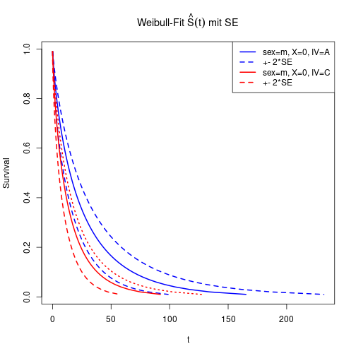
Detach (automatically) loaded packages (if possible)
try(detach(package:survival))
try(detach(package:splines))
Get the article source from GitHub
R markdown - markdown - R code - all posts