Multiple linear regression
TODO
- link to regressionDiag, regressionModMed, crossvalidation, resamplingBootALM
Install required packages
wants <- c("car", "leaps", "lmtest", "sandwich")
has   <- wants %in% rownames(installed.packages())
if(any(!has)) install.packages(wants[!has])
Descriptive model fit
Descriptive model fit
set.seed(123)
N  <- 100
X1 <- rnorm(N, 175, 7)
X2 <- rnorm(N,  30, 8)
X3 <- abs(rnorm(N, 60, 30))
Y  <- 0.5*X1 - 0.3*X2 - 0.4*X3 + 10 + rnorm(N, 0, 7)
dfRegr <- data.frame(X1, X2, X3, Y)
(fit12 <- lm(Y ~ X1 + X2, data=dfRegr))
Call:
lm(formula = Y ~ X1 + X2, data = dfRegr)

Coefficients:
(Intercept)           X1           X2
-47.5012 0.6805 -0.2965 lm(scale(Y) ~ scale(X1) + scale(X2), data=dfRegr)
Call:
lm(formula = scale(Y) ~ scale(X1) + scale(X2), data = dfRegr)

Coefficients:
(Intercept)    scale(X1)    scale(X2)
5.053e-16 2.972e-01 -1.568e-01 library(car)
scatter3d(Y ~ X1 + X2, fill=FALSE, data=dfRegr)
Estimated coefficients, residuals, and fitted values
coef(fit12)(Intercept) X1 X2
-47.5011799 0.6804857 -0.2964717 E <- residuals(fit12)
head(E) 1 2 3 4 5 6
-28.853937 -18.923898 -3.540015 -12.154867 3.585806 7.677999 Yhat <- fitted(fit12)
head(Yhat) 1 2 3 4 5 6
61.70483 60.98398 70.69952 63.84983 65.56255 70.96601 Add and remove predictors
(fit123 <- update(fit12, . ~ . + X3))
Call:
lm(formula = Y ~ X1 + X2 + X3, data = dfRegr)

Coefficients:
(Intercept)           X1           X2           X3
    19.1588       0.4445      -0.2596      -0.4134
(fit13 <- update(fit123, . ~ . - X1))
Call:
lm(formula = Y ~ X2 + X3, data = dfRegr)

Coefficients:
(Intercept)           X2           X3
    98.5347      -0.2763      -0.4261
(fit1 <- update(fit12, . ~ . - X2))
Call:
lm(formula = Y ~ X1, data = dfRegr)

Coefficients:
(Intercept)           X1
   -59.2628       0.6983
Assessing model fit
(Adjusted) \(R^{2}\) and residual standard error
sumRes <- summary(fit123)
sumRes$r.squared
[1] 0.7545767sumRes$adj.r.squared[1] 0.7469072sumRes$sigma[1] 7.360588Information criteria AIC and BIC
AIC(fit1)[1] 815.6499extractAIC(fit1)[1] 2.0000 529.8622extractAIC(fit1, k=log(N))[1] 2.0000 535.0725Crossvalidation
cv.glm() function from package boot, see crossvalidation
Coefficient tests and overall model test
summary(fit12)
Call:
lm(formula = Y ~ X1 + X2, data = dfRegr)

Residuals:
    Min      1Q  Median      3Q     Max
-31.857  -6.765   1.967   9.270  37.943

Coefficients:
            Estimate Std. Error t value Pr(>|t|)
(Intercept) -47.5012    39.0472  -1.217  0.22674
X1            0.6805     0.2187   3.112  0.00244 **
X2           -0.2965     0.1806  -1.641  0.10395
---
Signif. codes:  0 '***' 0.001 '**' 0.01 '*' 0.05 '.' 0.1 ' ' 1

Residual standard error: 13.89 on 97 degrees of freedom
Multiple R-squared:  0.1175,    Adjusted R-squared:  0.09931
F-statistic: 6.458 on 2 and 97 DF, p-value: 0.002328confint(fit12) 2.5 % 97.5 %
(Intercept) -124.9990783 29.99671860
X1 0.2464808 1.11449071
X2 -0.6549521 0.06200877vcov(fit12) (Intercept) X1 X2
(Intercept) 1524.684429 -8.455382007 -1.294237738
X1 -8.455382 0.047817791 0.001956354
X2 -1.294238 0.001956354 0.032623539Variable selection and model comparisons
Model comparisons
Effect of adding a single predictor
add1(fit1, . ~ . + X2 + X3, test="F")Single term additions
Model:
Y ~ X1
Df Sum of Sq RSS AIC F value Pr(>F)
<none> 19222 529.86
X2 1 519.5 18702 529.12 2.6942 0.104
X3 1 13622.6 5599 408.52 236.0033 <2e-16 ***
---
Signif. codes: 0 '***' 0.001 '**' 0.01 '*' 0.05 '.' 0.1 ' ' 1Effect of adding several predictors
anova(fit1, fit123)Analysis of Variance Table
Model 1: Y ~ X1
Model 2: Y ~ X1 + X2 + X3
Res.Df RSS Df Sum of Sq F Pr(>F)
1 98 19221.6
2 96 5201.1 2 14020 129.39 < 2.2e-16 ***
---
Signif. codes: 0 '***' 0.001 '**' 0.01 '*' 0.05 '.' 0.1 ' ' 1All predictor subsets
data(longley)
head(longley)
GNP.deflator GNP Unemployed Armed.Forces Population Year Employed
1947 83.0 234.289 235.6 159.0 107.608 1947 60.323
1948 88.5 259.426 232.5 145.6 108.632 1948 61.122
1949 88.2 258.054 368.2 161.6 109.773 1949 60.171
1950 89.5 284.599 335.1 165.0 110.929 1950 61.187
1951 96.2 328.975 209.9 309.9 112.075 1951 63.221
1952 98.1 346.999 193.2 359.4 113.270 1952 63.639library(leaps)
subs <- regsubsets(GNP.deflator ~ ., data=longley)
summary(subs, matrix.logical=TRUE)Subset selection object
Call: dwKnit(inputFile, outputFile, markdEngine, siteGen)
6 Variables (and intercept)
Forced in Forced out
GNP FALSE FALSE
Unemployed FALSE FALSE
Armed.Forces FALSE FALSE
Population FALSE FALSE
Year FALSE FALSE
Employed FALSE FALSE
1 subsets of each size up to 6
Selection Algorithm: exhaustive
GNP Unemployed Armed.Forces Population Year Employed
1 ( 1 ) TRUE FALSE FALSE FALSE FALSE FALSE
2 ( 1 ) FALSE FALSE TRUE FALSE TRUE FALSE
3 ( 1 ) TRUE TRUE FALSE TRUE FALSE FALSE
4 ( 1 ) TRUE TRUE TRUE TRUE FALSE FALSE
5 ( 1 ) TRUE TRUE TRUE TRUE TRUE FALSE
6 ( 1 ) TRUE TRUE TRUE TRUE TRUE TRUEplot(subs, scale="bic")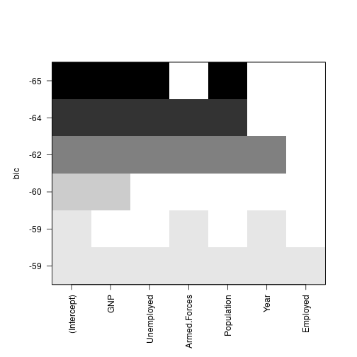
Xmat <- data.matrix(subset(longley, select=c("GNP", "Unemployed", "Population", "Year")))
(leapFits <- leaps(Xmat, longley$GNP.deflator, method="Cp"))
$which
1 2 3 4
1 TRUE FALSE FALSE FALSE
1 FALSE FALSE FALSE TRUE
1 FALSE FALSE TRUE FALSE
1 FALSE TRUE FALSE FALSE
2 FALSE TRUE FALSE TRUE
2 FALSE FALSE TRUE TRUE
2 TRUE FALSE FALSE TRUE
2 TRUE FALSE TRUE FALSE
2 TRUE TRUE FALSE FALSE
2 FALSE TRUE TRUE FALSE
3 TRUE TRUE TRUE FALSE
3 TRUE FALSE TRUE TRUE
3 FALSE TRUE TRUE TRUE
3 TRUE TRUE FALSE TRUE
4 TRUE TRUE TRUE TRUE
$label
[1] "(Intercept)" "1" "2" "3" "4"
$size
[1] 2 2 2 2 3 3 3 3 3 3 4 4 4 4 5
$Cp
[1] 9.934664 11.077014 42.000853 793.075625 8.960981 9.177695
[7] 9.430473 10.982967 10.985247 37.402418 3.000512 5.963360
[13] 8.781825 10.821894 5.000000plot(leapFits$size, leapFits$Cp, xlab="model size", pch=20, col="blue",
ylab="Mallows' Cp", main="Mallows' Cp agains model size")
abline(a=0, b=1)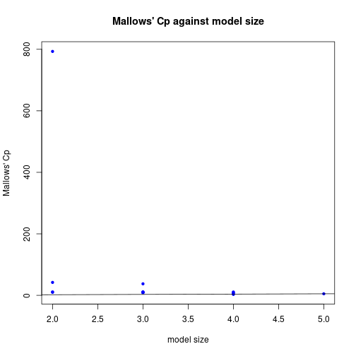
Apply regression model to new data
X1new <- c(177, 150, 192, 189, 181)
dfNew <- data.frame(X1=X1new)
predict(fit1, dfNew, interval="prediction", level=0.95)
fit lwr upr
1 64.33003 36.39261 92.26744
2 45.47689 15.38202 75.57176
3 74.80400 45.97114 103.63686
4 72.70920 44.17348 101.24492
5 67.12309 39.09370 95.15248predOrg <- predict(fit1, interval="confidence", level=0.95)hOrd <- order(X1)
par(lend=2)
plot(X1, Y, pch=20, xlab="Predictor", ylab="Dependent variable and prediction",
xaxs="i", main="Data and regression prediction")
polygon(c(X1[hOrd], X1[rev(hOrd)]),
c(predOrg[hOrd, "lwr"], predOrg[rev(hOrd), "upr"]),
border=NA, col=rgb(0.7, 0.7, 0.7, 0.6))
abline(fit1, col="black")
legend(x="bottomright", legend=c("Data", "prediction", "confidence region"),
pch=c(20, NA, NA), lty=c(NA, 1, 1), lwd=c(NA, 1, 8),
col=c("black", "blue", "gray"))
Detach (automatically) loaded packages (if possible)
try(detach(package:leaps))
try(detach(package:lmtest))
try(detach(package:sandwich))
try(detach(package:zoo))
try(detach(package:car))
Get the article source from GitHub
R markdown - markdown - R code - all posts