Regression diagnostics

TODO
Install required packages
Extreme values and outliers
- Univariate assessment of outliers
- Multivariate assessment of outliers
Leverage and influence
Checking model assumptions using residuals
Multicollinearity
Detach (automatically) loaded packages (if possible)
Get the article source from GitHub

TODO

link to regression, regressionLogistic

Install required packages

car, lmtest, mvoutlier, perturb, robustbase, tseries

wants <- c("car", "lmtest", "mvoutlier", "perturb", "robustbase", "tseries")
has   <- wants %in% rownames(installed.packages())
if(any(!has)) install.packages(wants[!has])

Extreme values and outliers

Univariate assessment of outliers

set.seed(123)
N  <- 100
X1 <- rnorm(N, 175, 7)
X2 <- rnorm(N,  30, 8)
X3 <- 0.3*X1 - 0.2*X2 + rnorm(N, 0, 5)
Y  <- 0.5*X1 - 0.3*X2 - 0.4*X3 + 10 + rnorm(N, 0, 5)
dfRegr <- data.frame(X1, X2, X3, Y)

library(robustbase)
xyMat <- data.matrix(dfRegr)
robXY <- covMcd(xyMat)
XYz   <- scale(xyMat, center=robXY$center, scale=sqrt(diag(robXY$cov)))
summary(XYz)

       X1                 X2                 X3                Y           
 Min.   :-2.53818   Min.   :-1.96554   Min.   :-2.4625   Min.   :-2.45112  
 1st Qu.:-0.63344   1st Qu.:-0.68918   1st Qu.:-0.5474   1st Qu.:-0.61660  
 Median :-0.05045   Median :-0.10278   Median : 0.1471   Median :-0.04010  
 Mean   :-0.02039   Mean   : 0.01779   Mean   : 0.1410   Mean   :-0.04869  
 3rd Qu.: 0.61065   3rd Qu.: 0.60431   3rd Qu.: 0.7874   3rd Qu.: 0.60444  
 Max.   : 2.17984   Max.   : 3.43113   Max.   : 2.9812   Max.   : 2.45654

Multivariate assessment of outliers

Mahalanobis distance with robust estimate for the covariance matrix

mahaSq <- mahalanobis(xyMat, center=robXY$center, cov=robXY$cov)
summary(sqrt(mahaSq))

   Min. 1st Qu.  Median    Mean 3rd Qu.    Max. 
 0.6179  1.3452  1.7461  1.8444  2.2515  3.9331

Nonparametric multivariate outlier detection with package mvoutlier

library(mvoutlier)
aqRes <- aq.plot(xyMat)

Projection to the first and second robust principal components.
Proportion of total variation (explained variance): 0.63336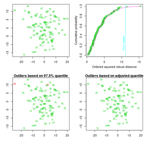

Where any outliers found?

which(aqRes$outliers)

integer(0)

Leverage and influence

fit <- lm(Y ~ X1 + X2 + X3, data=dfRegr)
h   <- hatvalues(fit)
summary(h)

   Min. 1st Qu.  Median    Mean 3rd Qu.    Max. 
0.01080 0.02190 0.03474 0.04000 0.05172 0.15248

cooksDst <- cooks.distance(fit)
summary(cooksDst)

     Min.   1st Qu.    Median      Mean   3rd Qu.      Max. 
8.300e-07 8.613e-04 3.650e-03 1.029e-02 1.362e-02 6.498e-02

inflRes <- influence.measures(fit)
summary(inflRes)

Potentially influential observations of
     lm(formula = Y ~ X1 + X2 + X3, data = dfRegr) :

   dfb.1_ dfb.X1 dfb.X2 dfb.X3 dffit cov.r   cook.d hat    
44 -0.04   0.05  -0.03  -0.02   0.06  1.15_*  0.00   0.09  
59  0.04  -0.04  -0.25   0.07  -0.38  0.83_*  0.03   0.02  
60  0.04   0.15  -0.20  -0.45   0.52  0.84_*  0.06   0.04  
64  0.05  -0.13   0.37   0.10   0.40  1.19_*  0.04   0.15_*
71  0.15  -0.20   0.02   0.17   0.34  0.84_*  0.03   0.02  
74  0.05  -0.02   0.11  -0.12   0.21  1.14_*  0.01   0.10  
95  0.04  -0.02   0.02  -0.07  -0.10  1.15_*  0.00   0.09  
97  0.16  -0.10  -0.09  -0.13  -0.20  1.16_*  0.01   0.12

library(car)
influenceIndexPlot(fit)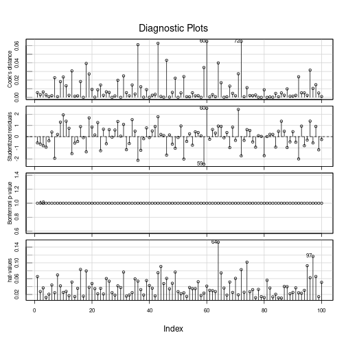

Checking model assumptions using residuals

Estnd <- rstandard(fit)
Estud <- rstudent(fit)

Normality assumption

par(mar=c(5, 4.5, 4, 2)+0.1)
hist(Estud, main="Histogram studentized residals", breaks="FD", freq=FALSE)
curve(dnorm(x, mean=0, sd=1), col="red", lwd=2, add=TRUE)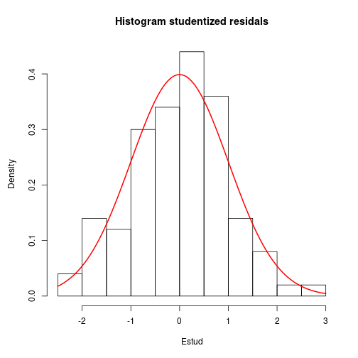

qqPlot(Estud, distribution="norm", pch=20, main="QQ-Plot studentized residuals")

[1] 60 59

qqline(Estud, col="red", lwd=2)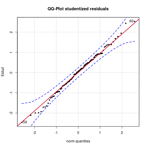

shapiro.test(Estud)


    Shapiro-Wilk normality test

data:  Estud
W = 0.99432, p-value = 0.9535

Independence and homoscedasticity assumption

Spread-level plot

library(car)
spreadLevelPlot(fit, pch=20)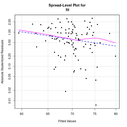


Suggested power transformation:  4.32355

Durbin-Watson-test for autocorrelation

library(car)
durbinWatsonTest(fit)

 lag Autocorrelation D-W Statistic p-value
   1     -0.08825048      2.172797   0.362
 Alternative hypothesis: rho != 0

Statistical tests for heterocedasticity

Breusch-Pagan-Test

library(lmtest)
bptest(fit)


    studentized Breusch-Pagan test

data:  fit
BP = 1.9213, df = 3, p-value = 0.5889

Score-test for non-constant error variance

library(car)
ncvTest(fit)

Non-constant Variance Score Test 
Variance formula: ~ fitted.values 
Chisquare = 0.548752, Df = 1, p = 0.45883

Linearity assumption

White-test

library(tseries)
white.test(dfRegr$X1, dfRegr$Y)


    White Neural Network Test

data:  dfRegr$X1 and dfRegr$Y
X-squared = 1.8307, df = 2, p-value = 0.4004

white.test(dfRegr$X2, dfRegr$Y)
white.test(dfRegr$X3, dfRegr$Y)
# not run

Response transformations

lamObj  <- powerTransform(fit, family="bcPower")
(lambda <- coef(lamObj))

      Y1 
1.280836

library(car)
yTrans <- bcPower(dfRegr$Y, lambda)

Multicollinearity

Pairwise correlations between predictor variables

X   <- data.matrix(subset(dfRegr, select=c("X1", "X2", "X3")))
(Rx <- cor(X))

            X1          X2         X3
X1  1.00000000 -0.04953215  0.2700393
X2 -0.04953215  1.00000000 -0.2929049
X3  0.27003928 -0.29290486  1.0000000

Variance inflation factor

library(car)
vif(fit)

      X1       X2       X3 
1.079770 1.094974 1.178203

Condition indexes

\(\kappa\)

fitScl <- lm(scale(Y) ~ scale(X1) + scale(X2) + scale(X3), data=dfRegr)
kappa(fitScl, exact=TRUE)

[1] 1.508749

library(perturb)
colldiag(fit, scale=TRUE, center=TRUE)

Condition
Index   Variance Decomposition Proportions
         X1    X2    X3   
1  1.000 0.162 0.181 0.280
2  1.224 0.528 0.440 0.000
3  1.509 0.311 0.379 0.720

Using package `perturb`

pRes <- perturb(fit, pvars=c("X1", "X2", "X3"), prange=c(1, 1, 1))
summary(pRes)

$formula
[1] "Y ~ X1 + X2 + X3"

$pvars
[1] "X1" "X2" "X3"

$prange
[1] 1 1 1

$ptrans2
character(0)

$formula2
[1] "Y ~ X1.1 + X2.1 + X3.1"

$distribution
[1] "normal"

$summ
                  mean       s.d.        min        max
(Intercept) 17.4182516 2.74597430 10.5755610 23.9483451
X1           0.4616296 0.01774141  0.4149206  0.5012884
X2          -0.2734070 0.01414048 -0.3074216 -0.2358462
X3          -0.4342440 0.02780265 -0.5184953 -0.3792446

$dec.places
[1] 3

$full
[1] FALSE

$dots
[1] ""

attr(,"class")
[1] "summary.perturb"

Detach (automatically) loaded packages (if possible)

try(detach(package:tseries))
try(detach(package:lmtest))
try(detach(package:zoo))
try(detach(package:perturb))
try(detach(package:mvoutlier))
try(detach(package:robustbase))
try(detach(package:sgeostat))
try(detach(package:car))
try(detach(package:carData))

Get the article source from GitHub

R markdown - markdown - R code - all posts