Binary logistic regression
TODO
- link to associationOrder for
pROC, regressionOrdinal, regressionMultinom, regressionDiag for outliers, collinearity, crossvalidation
Install required packages
wants <- c("rms")
has   <- wants %in% rownames(installed.packages())
if(any(!has)) install.packages(wants[!has])
Descriptive model fit
Simulate data
set.seed(123)
SSRIpre  <- c(18, 16, 16, 15, 14, 20, 14, 21, 25, 11)
SSRIpost <- c(12,  0, 10,  9,  0, 11,  2,  4, 15, 10)
PlacPre  <- c(18, 16, 15, 14, 20, 25, 11, 25, 11, 22)
PlacPost <- c(11,  4, 19, 15,  3, 14, 10, 16, 10, 20)
WLpre    <- c(15, 19, 10, 29, 24, 15,  9, 18, 22, 13)
WLpost   <- c(17, 25, 10, 22, 23, 10,  2, 10, 14,  7)

P        <- 3
Nj       <- rep(length(SSRIpre), times=P)
IV       <- factor(rep(1:P, Nj), labels=c("SSRI", "Placebo", "WL"))
DVpre    <- c(SSRIpre,  PlacPre,  WLpre)
DVpost   <- c(SSRIpost, PlacPost, WLpost)
postFac  <- cut(DVpost, breaks=c(-Inf, median(DVpost), Inf),
                        labels=c("lo", "hi"))
dfAncova <- data.frame(IV, DVpre, DVpost, postFac)cdplot(postFac ~ DVpre, data=dfAncova, subset=IV == "SSRI",
main="Estimated categ probs SSRI")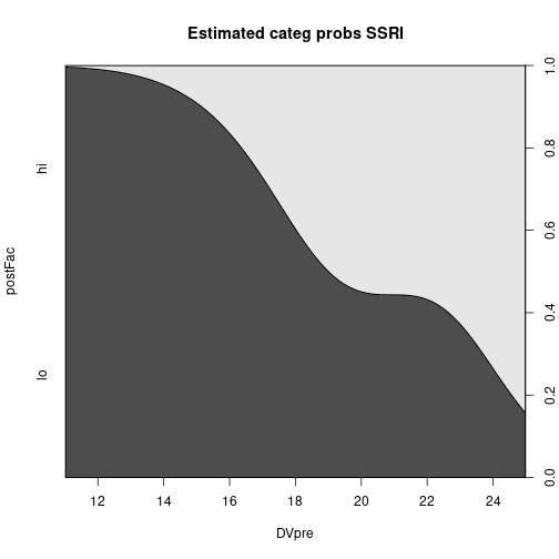
cdplot(postFac ~ DVpre, data=dfAncova, subset=IV == "Placebo",
       main="Estimated categ probs placebo")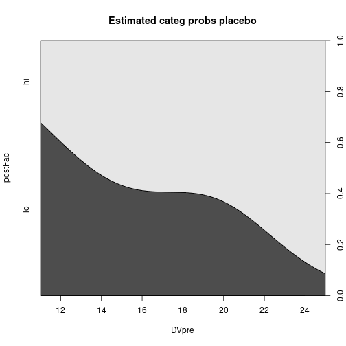
cdplot(postFac ~ DVpre, data=dfAncova, subset=IV == "WL",
       main="Estimated categ probs WL")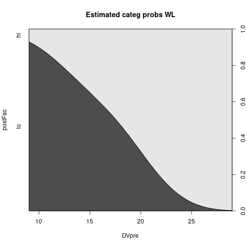
Fit the model
(glmFit <- glm(postFac ~ DVpre + IV, family=binomial(link="logit"), data=dfAncova))
Call:  glm(formula = postFac ~ DVpre + IV, family = binomial(link = "logit"),
    data = dfAncova)

Coefficients:
(Intercept)        DVpre    IVPlacebo         IVWL
    -8.4230       0.4258       1.7306       1.2027

Degrees of Freedom: 29 Total (i.e. Null);  26 Residual
Null Deviance:      41.46
Residual Deviance: 24.41    AIC: 32.41
Odds ratios
exp(coef(glmFit)) (Intercept) DVpre IVPlacebo IVWL
0.0002197532 1.5308001795 5.6440022784 3.3291484767 Profile likelihood based confidence intervals for odds ratios
exp(confint(glmFit)) 2.5 % 97.5 %
(Intercept) 1.488482e-07 0.0251596
DVpre 1.193766e+00 2.2446549
IVPlacebo 5.343091e-01 95.1942030
IVWL 2.916673e-01 52.2883653Fit the model based on a matrix of counts
N      <- 100
x1     <- rnorm(N, 100, 15)
x2     <- rnorm(N, 10, 3)
total  <- sample(40:60, N, replace=TRUE)
hits   <- rbinom(N, total, prob=0.4)
hitMat <- cbind(hits, total-hits)
glm(hitMat ~ x1 + x2, family=binomial(link="logit"))
Call:  glm(formula = hitMat ~ x1 + x2, family = binomial(link = "logit"))

Coefficients:
(Intercept)           x1           x2
  -0.102410    -0.003373     0.005638

Degrees of Freedom: 99 Total (i.e. Null);  97 Residual
Null Deviance:      99.35
Residual Deviance: 96.44    AIC: 532.5
Fit the model based on relative frequencies
relHits <- hits/total
glm(relHits ~ x1 + x2, weights=total, family=binomial(link="logit"))
Call:  glm(formula = relHits ~ x1 + x2, family = binomial(link = "logit"),
    weights = total)

Coefficients:
(Intercept)           x1           x2
  -0.102410    -0.003373     0.005638

Degrees of Freedom: 99 Total (i.e. Null);  97 Residual
Null Deviance:      99.35
Residual Deviance: 96.44    AIC: 532.5
Fitted logits and probabilities
logitHat <- predict(glmFit, type="link")
plot(logitHat, pch=16, col=c("red", "blue")[unclass(dfAncova$postFac)])
abline(h=0)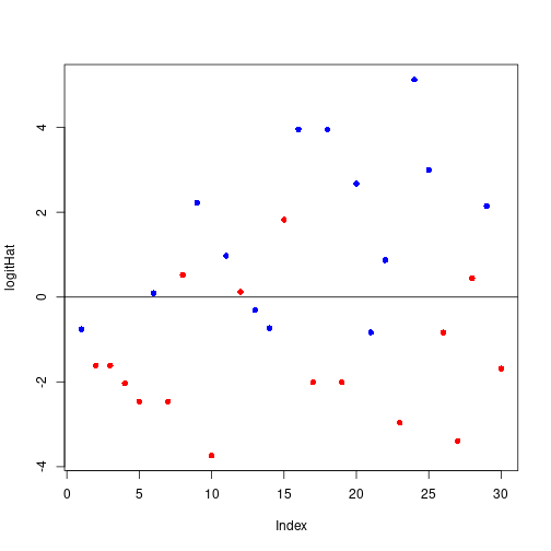
Phat <- fitted(glmFit)
Phat <- predict(glmFit, type="response")
head(Phat)
1 2 3 4 5 6
0.31891231 0.16653918 0.16653918 0.11545968 0.07856997 0.52318493 mean(Phat)[1] 0.4666667prop.table(xtabs(~ postFac, data=dfAncova))postFac
lo hi
0.5333333 0.4666667 Assess model fit
Classification table
thresh <- 0.5
facHat <- cut(Phat, breaks=c(-Inf, thresh, Inf), labels=c("lo", "hi"))
cTab   <- xtabs(~ postFac + facHat, data=dfAncova)
addmargins(cTab)
facHat
postFac lo hi Sum
lo 12 4 16
hi 4 10 14
Sum 16 14 30Correct classification rate
(CCR <- sum(diag(cTab)) / sum(cTab))[1] 0.7333333log-Likelihood, AUC, Somers’ \(D_{xy}\), Nagelkerke’s pseudo \(R^{2}\)
Deviance, log-likelihood and AIC
deviance(glmFit)[1] 24.40857logLik(glmFit)'log Lik.' -12.20428 (df=4)AIC(glmFit)[1] 32.40857Nagelkerke’s pseudo-\(R^{2}\) (R2), area under the ROC-Kurve (C), Somers’ \(D_{xy}\) (Dxy), Goodman & Kruskal’s \(\gamma\) (Gamma), Kendall’s \(\tau\) (Tau-a)
library(rms)
lrm(postFac ~ DVpre + IV, data=dfAncova)
Logistic Regression Model

lrm(formula = postFac ~ DVpre + IV, data = dfAncova)

                     Model Likelihood     Discrimination    Rank Discrim.
                        Ratio Test            Indexes          Indexes
Obs            30    LR chi2     17.05    R2       0.579    C       0.900
 lo            16    d.f.            3    g        2.686    Dxy     0.799
 hi            14    Pr(> chi2) 0.0007    gr      14.672    gamma   0.803
max |deriv| 2e-06                         gp       0.404    tau-a   0.411
                                          Brier    0.139

           Coef    S.E.   Wald Z Pr(>|Z|)
Intercept  -8.4230 2.9502 -2.86  0.0043
DVpre       0.4258 0.1553  2.74  0.0061
IV=Placebo  1.7306 1.2733  1.36  0.1741
IV=WL       1.2027 1.2735  0.94  0.3450
For plotting the ROC-curve, see pROC in associationOrder
McFadden, Cox & Snell and Nagelkerke pseudo \(R^{2}\)
Log-likelihoods for full model and 0-model without predictors X1, X2
N    <- nobs(glmFit)
glm0 <- update(glmFit, . ~ 1)
LLf  <- logLik(glmFit)
LL0  <- logLik(glm0)
McFadden pseudo-\(R^2\)
as.vector(1 - (LLf / LL0))[1] 0.411209Cox & Snell
as.vector(1 - exp((2/N) * (LL0 - LLf)))[1] 0.4334714Nagelkerke
as.vector((1 - exp((2/N) * (LL0 - LLf))) / (1 - exp(LL0)^(2/N)))[1] 0.578822Crossvalidation
cv.glm() function from package boot, see crossvalidation
Apply model to new data
Nnew  <- 3
dfNew <- data.frame(DVpre=rnorm(Nnew, 20, sd=7),
                    IV=factor(rep("SSRI", Nnew), levels=levels(dfAncova$IV)))
predict(glmFit, newdata=dfNew, type="response")
1 2 3
0.11516886 0.10427434 0.06270597 Coefficient tests and overall model test
Individual coefficient tests
Wald-tests for parameters
summary(glmFit)
Call:
glm(formula = postFac ~ DVpre + IV, family = binomial(link = "logit"),
    data = dfAncova)

Deviance Residuals:
    Min       1Q   Median       3Q      Max
-1.9865  -0.5629  -0.2372   0.4660   1.5455

Coefficients:
            Estimate Std. Error z value Pr(>|z|)
(Intercept)  -8.4230     2.9502  -2.855   0.0043 **
DVpre         0.4258     0.1553   2.742   0.0061 **
IVPlacebo     1.7306     1.2733   1.359   0.1741
IVWL          1.2027     1.2735   0.944   0.3450
---
Signif. codes:  0 '***' 0.001 '**' 0.01 '*' 0.05 '.' 0.1 ' ' 1

(Dispersion parameter for binomial family taken to be 1)

    Null deviance: 41.455  on 29  degrees of freedom
Residual deviance: 24.409  on 26  degrees of freedom
AIC: 32.409

Number of Fisher Scoring iterations: 5
Or see lrm() above
Model comparisons - likelihood-ratio tests
anova(glm0, glmFit, test="Chisq")Analysis of Deviance Table
Model 1: postFac ~ 1
Model 2: postFac ~ DVpre + IV
Resid. Df Resid. Dev Df Deviance Pr(>Chi)
1 29 41.455
2 26 24.409 3 17.047 0.0006912 ***
---
Signif. codes: 0 '***' 0.001 '**' 0.01 '*' 0.05 '.' 0.1 ' ' 1drop1(glmFit, test="Chi")Single term deletions
Model:
postFac ~ DVpre + IV
Df Deviance AIC LRT Pr(>Chi)
<none> 24.409 32.409
DVpre 1 39.540 45.540 15.1319 0.0001003 ***
IV 2 26.566 30.566 2.1572 0.3400666
---
Signif. codes: 0 '***' 0.001 '**' 0.01 '*' 0.05 '.' 0.1 ' ' 1Or see lrm() above
Model comparisons for testing IV
glmPre <- update(glmFit, . ~ . - IV) # no IV factor
anova(glmPre, glmFit, test="Chisq")
Analysis of Deviance Table
Model 1: postFac ~ DVpre
Model 2: postFac ~ DVpre + IV
Resid. Df Resid. Dev Df Deviance Pr(>Chi)
1 28 26.566
2 26 24.409 2 2.1572 0.3401Model comparisons for testing DVpre
anova(glm0, glmPre, test="Chisq")Analysis of Deviance Table
Model 1: postFac ~ 1
Model 2: postFac ~ DVpre
Resid. Df Resid. Dev Df Deviance Pr(>Chi)
1 29 41.455
2 28 26.566 1 14.89 0.000114 ***
---
Signif. codes: 0 '***' 0.001 '**' 0.01 '*' 0.05 '.' 0.1 ' ' 1Further resources
For penalized logistic regression, see packages logistf (using Firth’s penalized likelihood) and glmnet. An example using glmnet for linear regression is in regressionRobPen.
Detach (automatically) loaded packages (if possible)
try(detach(package:rms))
try(detach(package:Hmisc))
try(detach(package:grid))
try(detach(package:lattice))
try(detach(package:survival))
try(detach(package:splines))
try(detach(package:Formula))
Get the article source from GitHub
R markdown - markdown - R code - all posts