Customize diagrams: Add additional elements

TODO

• link to diagDevice for regions, diagFormat, diagScatter

Install required packages

Hmisc, mvtnorm, plotrix

wants <- c("Hmisc", "mvtnorm", "plotrix")
has   <- wants %in% rownames(installed.packages())
if(any(!has)) install.packages(wants[!has])

Identify coordinates in scatterplots

To later add elements to the plot

vec <- rnorm(10)
plot(vec, pch=16)
(xy <- locator(n=3))

$x
[1] 4.952304 7.076921 2.068896

$y
[1] 0.09391669 -0.13407651 -0.88645406

Add elements to arbitrary device regions

Each device has its own coordinate system.

library(Hmisc)
set.seed(123)
par(xpd=NA, mar=c(5, 5, 5, 5))
plot(rnorm(10), xlab=NA, ylab=NA, pch=20)
pt1 <- cnvrt.coords(0, 0, input="fig")
pt1$usr

$x
[1] -1.304

$y
[1] -2.027974

points(pt1$usr$x + 0.5, pt1$usr$y + 0.3, pch=4, lwd=5, cex=5, col="darkgray")
text(pt1$usr$x + 1, pt1$usr$y + 0.24, adj=c(0, 0), 
     labels="cross lower-left figure-region", cex=1.5)
pt2 <- cnvrt.coords(c(0.05, 0.95), c(0.95, 0.05), input="tdev")
pt2$usr

$x
[1] -0.6236 11.6236

$y
[1]  2.252680 -1.802676

arrows(x0=pt2$usr$x[1], y0=pt2$usr$y[1],
       x1=pt2$usr$x[2], y1=pt2$usr$y[2], lwd=4, code=3,
       angle=90, lend=2, col="darkgray")
text(pt2$usr$x[1] + 0.5, pt2$usr$y[1], adj=c(0, 0),
     labels="arrow across total device-region", cex=1.5)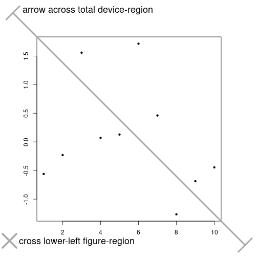

Points and lines

Points and lines

xA <- seq(-15, 15, length.out=200)
yA <- sin(xA) / xA                ## sinc function
plot(xA, yA, type="l", xlab="x", ylab="sinc(x)",
     main="Add points and lines", lwd=2)
abline(h=0, col="darkgreen", lwd=2)

idx <- round(seq(1, length(xA), length.out=30))
points(xA[idx], yA[idx], col="red", pch=16, cex=1.5)
yB <- sin(pi * xA) / (pi * xA)    ## normalized sinc function
lines(xA, yB, col="blue", type="l", lwd=2)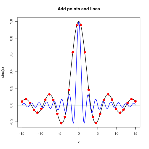

Gridlines, line segments, and arrows

X    <- rnorm(20, 175, 7)
Y    <- 0.5*X + 10 + rnorm(20, 0, 4)
fit  <- lm(Y ~ X)
pred <- fitted(fit)

par(lend=2)
plot(Y ~ X, asp=1, type="n", main="Add grid, line segments and arrows")
abline(fit, lwd=2)
grid(lwd=2, col="gray")
segments(x0=X, y0=pred, x1=X, y1=Y, lwd=2, col="darkgray")
arrows(x0=c(X[1]-6,   X[3]),
       y0=c(Y[1],     Y[3]+6),
       x1=c(X[1]-0.5, X[3]),
       y1=c(Y[1],     Y[3]+0.5),
       col="red", lwd=2)
arrows(x0=X[4]+0.1*(X[7]-X[4]),
       y0=Y[4]+0.1*(Y[7]-Y[4]),
       x1=X[4]+0.9*(X[7]-X[4]),
       y1=Y[4]+0.9*(Y[7]-Y[4]), code=3, col="red", lwd=2)
points(Y ~ X, pch=16, cex=1.5, col="blue")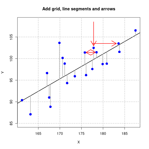

Rectangles, polygons, and text

Rectangles and text

n      <- 7
len    <- 1/n
colsR  <- rep(seq(0.9, 0.2, length.out=n),  each=n)
colsG  <- rep(seq(0.9, 0.2, length.out=n), times=n)
cols   <- rgb(colsR, colsG, 0)
xLeft  <- rep(seq(0,   1-len, by=len), times=n)
yBot   <- rep(seq(0,   1-len, by=len),  each=n)
xRight <- rep(seq(len, 1,     by=len), times=n)
yTop   <- rep(seq(len, 1,     by=len),  each=n)

plot(c(0, 1), c(0, 1), axes=FALSE, xlab=NA, ylab=NA, type="n",
     asp=1, main="Color ramp")
rect(xLeft, yBot, xRight, yTop, border=NA, col=cols)
idx   <- c(10, 27)
xText <- xLeft[idx] + (xRight[idx]-xLeft[idx])/2
yText <- yBot[idx]  + (yTop[idx]  - yBot[idx])/2
text(xText, yText, labels=cols[idx])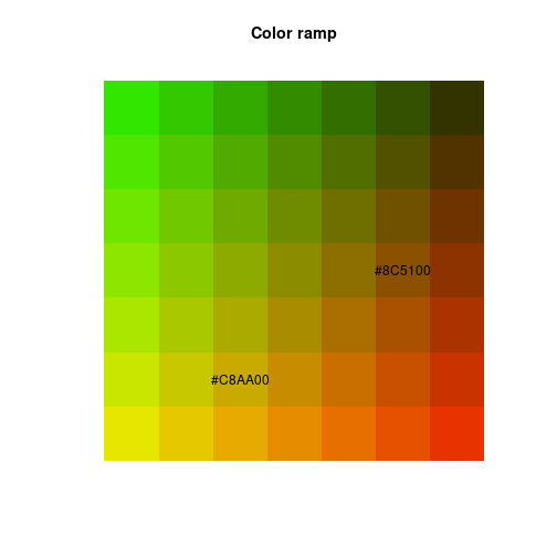

Polygons, mathematical symbols, and custom axes

Filled polygon

mu    <- 0
sigma <- 3
xLims <- c(mu-4*sigma, mu+4*sigma)
X     <- seq(xLims[1], xLims[2], length.out=100)
Y     <- dnorm(X, mu, sigma)
selX  <- seq(mu-sigma, mu+sigma, length.out=100)
selY  <- dnorm(selX, mu, sigma)
cdf   <- pnorm(X, mu, sigma)

par(mar=c(5, 4, 4, 5), cex.lab=1.4)
plot(X, Y, type="n", xlim=xLims-c(-2, 2), xlab=NA, ylab=NA,
     main="Normal PDF and CDF N(0, 3)")
box(which="plot", col="gray", lwd=2)
polygon(c(selX, rev(selX)), c(selY, rep(-1, length(selX))),
        border=NA, col="lightgray")
lines(X, Y, lwd=2)
par(new=TRUE)
plot(X, cdf, xlim=xLims-c(-2, 2), type="l", lwd=2, col="blue", xlab="x",
     ylab=NA, axes=FALSE)
axis(side=4, at=seq(0, 1, by=0.1), col="blue")
segments(x0=c(mu-sigma, mu, mu+sigma),
         y0=c(-1, -1, -1),
         x1=c(mu-sigma, mu, mu+sigma),
         y1=c(pnorm(mu-sigma, mu, sigma), pnorm(mu, mu, sigma),
              pnorm(mu+sigma, mu, sigma)),
         lwd=2, col=c("darkgreen", "red", "darkgreen"), lty=2)
segments(x0=c(mu-sigma, mu, mu+sigma),
         y0=c(pnorm(mu-sigma, mu, sigma), pnorm(mu, mu, sigma),
              pnorm(mu+sigma, mu, sigma)),
         x1=xLims[2]+10,
         y1=c(pnorm(mu-sigma, mu, sigma), pnorm(mu, mu, sigma),
              pnorm(mu+sigma, mu, sigma)),
         lwd=2, col=c("darkgreen", "red", "darkgreen"), lty=2)
arrows(x0=c(mu-sigma+0.2, mu+sigma-0.2), y0=-0.02,
       x1=c(mu-0.2, mu+0.2),             y1=-0.02,
       code=3, angle=90, length=0.05, lwd=2, col="darkgreen")
mtext(text="F(x)", side=4, line=3, cex=1.4)
rect(-8.5, 0.92, -5.5, 1.0, col="lightgray", border=NA)
text(-7.2, 0.9, labels="probability")
text(-7.1, 0.86, expression(of~interval~group("[", list(-sigma, sigma), "]")))
text(mu-sigma/2, 0,    expression(sigma), col="darkgreen", cex=1.2)
text(mu+sigma/2, 0,    expression(sigma), col="darkgreen", cex=1.2)
text(mu+0.5,     0.02, expression(mu),    col="red",       cex=1.2)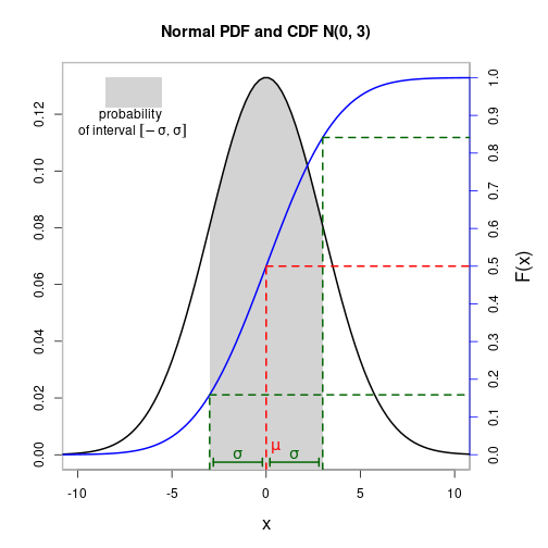

Polygon with shading lines

N      <- 10
muH0   <- 0
muH1   <- 1.6
alpha  <- 0.05
sigma  <- 2

(d <- (muH1-muH0) / sigma)

[1] 0.8

(delta <- (muH1-muH0) / (sigma/sqrt(N)))

[1] 2.529822

(tCrit <- qt(1-alpha, N-1))

[1] 1.833113

(powT <- 1-pt(tCrit, N-1, delta))

[1] 0.7544248

xLims <- c(-5, 10)

tLeft  <- seq(xLims[1], tCrit, length.out=100)
tRight <- seq(tCrit, xLims[2], length.out=100)
yH0r   <- dt(tRight, N-1, 0)
yH1l   <- dt(tLeft,  N-1, delta)
yH1r   <- dt(tRight, N-1, delta)

curve(dt(x, N-1, 0), xlim=xLims, ylim=c(0, 0.4), lwd=2, col="red",
      xlab="t", ylab="probability density",
      main="t distribution under H0 und H1", xaxs="i")
curve(dt(x, N-1, delta), lwd=2, col="blue", add=TRUE)
polygon(c(tRight, rev(tRight)), c(yH0r, numeric(length(tRight))),
        border=NA, col=rgb(1, 0.3, 0.3, 0.6))
polygon(c(tLeft, rev(tLeft)),  c(yH1l, numeric(length(tLeft))),
        border=NA, col=rgb(0.3, 0.3, 1, 0.6))
polygon(c(tRight, rev(tRight)), c(yH1r, numeric(length(tRight))),
        border=NA, density=5, lty=2, lwd=2, angle=45, col="darkgray")
abline(v=tCrit, lty=1, lwd=3, col="red")
text(tCrit+0.2, 0.4,  adj=0, labels="critical value")
text(tCrit-2.5, 0.38, adj=1, labels="distribution under H0")
text(tCrit+2,   0.2,  adj=0, labels="distribution under H1")
text(tCrit+1.0, 0.08, adj=0, labels="power")
text(tCrit-0.7, 0.05,  expression(beta))
text(tCrit+0.5, 0.015, expression(alpha))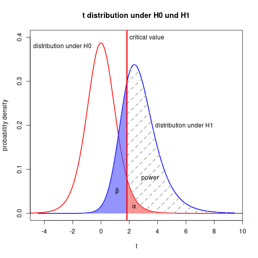

As opposed to polygon(), function polypath() can draw polygons with holes.

Function curves and mathematical symbols

mu    <- 0
sigma <- 2
curve(dnorm(x, mean=1, sd=1), from=-7, to=7, col="blue", lwd=2, cex.lab=1.4)
curve((1/(sigma*sqrt(2*pi))) * exp(-0.5*(((x-mu)/sigma)^2)), add=TRUE, lwd=2, lty=2)
title(main="Two normal PDF curves", sub="sub-title")
legend(x="topleft", legend=c("N(1, 1)", "N(0, 2)"), col=c("blue", "black"),
       lty=c(1, 2))
text(x=3.6,  y=0.35, labels="normal distribution\nN(1, 1)")
text(x=-3.5, y=0.1 , labels="N(0, 2)")
mtext(text="Probability density", side=3)
text(-4, 0.3, expression(frac(1, sigma*sqrt(2*pi))~exp*bgroup("(", -frac(1, 2)~bgroup("(", frac(x-mu, sigma), ")")^2, ")")))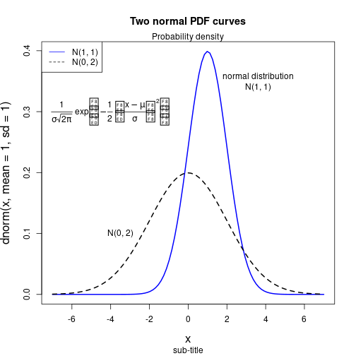

See ?plotmath and demo(plotmath) for explanations and further demos for mathematical expressions.

Custom axes, custom grid, and plot legend

vec <- seq(from=-2*pi, to=2*pi, length.out=200)
mat <- cbind(sin(vec), cos(vec))
pts <- tan(vec)
pts <- ifelse(abs(pts) > 2, NA, pts)
idx <- round(seq(0, length(vec), length.out=100))

matplot(vec, mat, ylim=c(-2, 2), lwd=2, col=c(12, 14),
        type="l", lty=1, xaxt="n", xlab=NA, ylab=NA,
        main="Trigonometric functions")
points(vec[idx], pts[idx], pch=16, cex=1.5, col=17)
xTicks  <- seq(from=-2*pi, to=2*pi, by=pi/2)
xLabels <- c("-2*pi", "-3*pi/2", "-pi", "-pi/2", "0", "pi/2", "pi", "3*pi/2", "2*pi")
axis(side=1, at=xTicks, labels=xLabels)
abline(h=c(-1, 0, 1), v=seq(from=-3*pi/2, to=3*pi/2, by=pi/2), col="gray", lty=3, lwd=2)
abline(h=0, v=0, lwd=2)
legend(x="bottomleft", legend=c("sin(x)", "cos(x)", "tan(x)"), cex=1.3,
       lty=c(1, 1, NA), pch=c(NA, NA, 16), col=c(12, 14, 17), bg="white")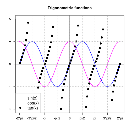

Error bars

Simulate data

Nj <- c(15, 20, 18, 22)
P  <- length(Nj)
DV <- rnorm(sum(Nj), rep(c(30, 20, 25, 15), Nj), 8)
IV <- factor(rep(1:P, Nj))
Mj <- tapply(DV, IV, FUN=mean)
Sj <- tapply(DV, IV, FUN=sd)
ciWidths <- qt(0.975, df=Nj-1) * Sj / sqrt(Nj)

Using plotCI() from package plotrix

library(plotrix)
stripchart(DV ~ IV, method="jitter", xlab="Group",
           main="Data und confidence intervals", xaxt="n",
           col="darkgray", ylim=c(0, 40), pch=16, vert=TRUE)
plotCI(x=Mj, uiw=ciWidths, sfrac=0, col="blue",
       cex=2, lwd=3, pch=16, add=TRUE)
axis(side=1, at=1:P, labels=LETTERS[1:P])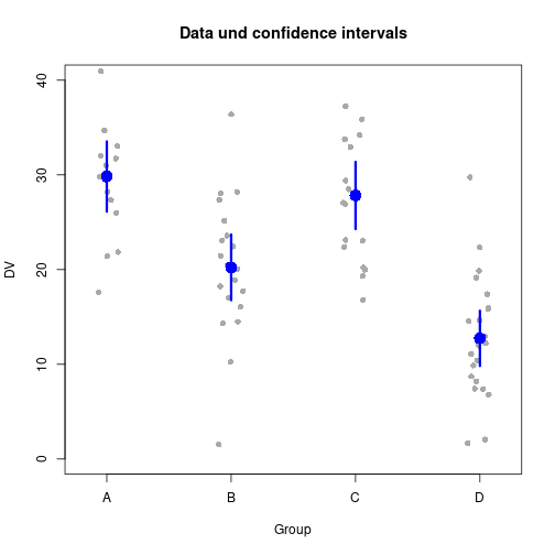

Means and error bars in a two-way design

Mj1 <- c(2, 3, 6, 3, 5)
Sj1 <- c(1.7, 1.8, 1.7, 1.9, 1.8)
Mj2 <- c(4, 3, 2, 1, 3)
Sj2 <- c(1.4, 1.7, 1.7, 1.3, 1.5)
Q   <- length(Mj1)

xOff <- 0.1
plotCI(y=c(Mj1, Mj2), x=c((1:Q)-xOff, (1:Q)+xOff), uiw=c(Sj1, Sj2),
       xlab="Factor A", ylab="Means", ylim=c(0, 8),
       main="Means and SDs in a 5x2 Design", pch=20, cex=2, lwd=2,
       col=rep(c("blue", "red"), each=5), lty=rep(1:2, each=Q))
legend(x="topleft", legend=c("B-1", "B-2"), pch=c(19, 19),
       col=c("blue", "red"))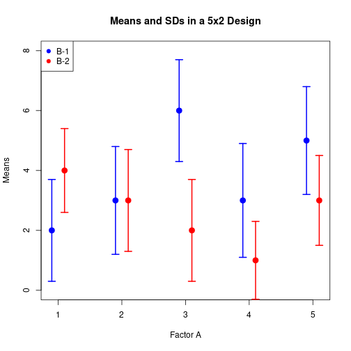

Using arrows()

barsX <- barplot(height=Mj, ylim=c(0, 40), xaxt="n", xlab="Group",
                 ylab="Means", main="Means and confidence intervals")
axis(side=1, at=barsX, labels=LETTERS[1:P])
limHi <- Mj + ciWidths
limLo <- Mj - ciWidths
arrows(x0=barsX, y0=limLo, x1=barsX, y1=limHi, code=3, angle=90,
       length=0.1, col="blue", lwd=2)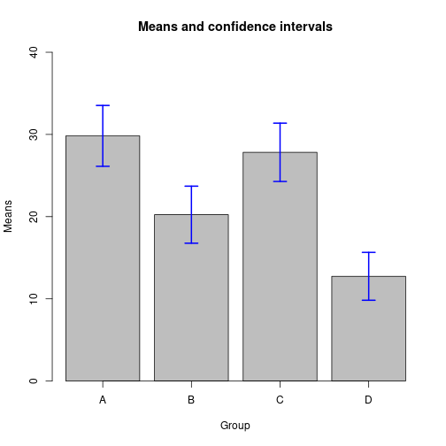

Raster images

See packages imager or adimpro to read in image files of various formats.

2-D color ramp square pattern

pxSq  <- 6
colsR <- rep(0.4, pxSq^2)
colsG <- rep(seq(0, 1, length.out=pxSq), times=pxSq)
colsB <- rep(seq(0, 1, length.out=pxSq), each=pxSq)
arrSq <- array(c(colsR, colsG, colsB), c(pxSq, pxSq, 3))
sqIm  <- as.raster(arrSq)

Gabor patch: oriented 2-D cosine with contrast following a 2-D normal distribution

pxG    <- 500
alpha  <- 0.4
beta   <- min(1-alpha, 1+alpha)
freq   <- 3
vals   <- rep(seq(-2*pi, 2*pi, length.out=pxG), pxG)
x      <- matrix(vals, nrow=pxG, byrow=TRUE)
y      <- matrix(vals, nrow=pxG, byrow=FALSE)
phi    <- alpha*x + beta*y
cosMat <- 0.5*cos(freq*phi) + 0.5

library(mvtnorm)
mu       <- c(0, 0)
sigma    <- diag(2)*9
gaussVal <- dmvnorm(cbind(c(x), c(y)), mu, sigma)
gaussMat <- matrix(gaussVal, nrow=pxG) / max(gaussVal)
gabIm    <- as.raster(cosMat*gaussMat)

plot(c(0, 1), c(0, 1), type="n", main="Bitmaps", xlab="", ylab="", asp=1)
rasterImage(sqIm,  0,   0,   0.4, 0.4, angle=0,  interpolate=FALSE)
rasterImage(gabIm, 0.5, 0.3, 1.1, 0.9, angle=10, interpolate=TRUE)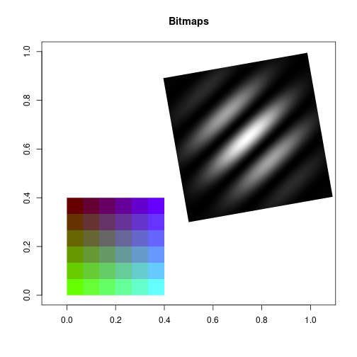

Detach (automatically) loaded packages (if possible)

try(detach(package:Hmisc))
try(detach(package:survival))
try(detach(package:lattice))
try(detach(package:Formula))
try(detach(package:ggplot2))
try(detach(package:mvtnorm))
try(detach(package:plotrix))

Get the article source from GitHub

R markdown - markdown - R code - all posts