Customize diagrams: Formatting
TODO
- link to diagAddElements ->
axis(), diagMultiple
Install required packages
wants <- c("RColorBrewer")
has   <- wants %in% rownames(installed.packages())
if(any(!has)) install.packages(wants[!has])
Formatting elements for all kinds of diagrams
Nearly all R base diagrams come with a shared set of options to control typical diagram elements like the title, axis labels and limits, or the type of plot symbol. They are illustrated here using the plot() function for simple scatter plots.
Plot symbols and line types
Plot symbols are chosen with option pch.
X <- row(matrix(numeric(6*5), nrow=6, ncol=5))
Y <- col(matrix(numeric(6*5), nrow=6, ncol=5))

par(mar=c(1, 1, 4, 2))
plot(0:5, seq(1, 5, length.out=6), type="n", xlab=NA, ylab=NA,
     axes=FALSE, main="Data symbols")
points(X[1:26], Y[1:26], pch=0:25, bg="gray", cex=3)
text(X[1:26]-0.3, Y[1:26], labels=0:25)
text(0.2, 3, labels="symbols for pch", srt=90, cex=1.2)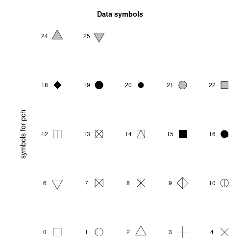
Line types are chosen with option lty, line widths with option lwd, and round vs. square line ends with lend.
X <- row(matrix(numeric(6*12), nrow=6, ncol=12))
Y <- col(matrix(numeric(6*12), nrow=6, ncol=12))

par(mar=c(1, 1, 4, 2))
plot(0:6, seq(1, 12, length.out=7), type="n", axes=FALSE)
matlines(X[ , 1:6],  Y[ , 1:6],  lty=6:1, lwd=6:1, lend=0, col="blue")
matlines(X[ , 7:12], Y[ , 7:12], lty=6:1, lwd=6:1, lend=1, col="black")

## add annotations
text(rep(0.7, 12), Y[1, 1:12], labels=c(6:1, 6:1))
text(0, 7, labels="line types: lty, line widths: lwd", srt=90, cex=1.2)
text(0.32, 9, labels="line ending: lend=1", srt=90, cex=1.2)
text(0.32, 3, labels="line ending: lend=0", srt=90, cex=1.2)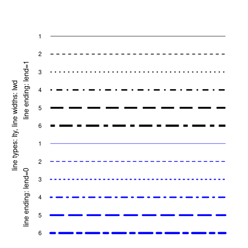
Diagram title, axis labels, axis limits, aspect ratio
set.seed(123)
N <- 100
x <- rnorm(N, 100, 15)
y <- 0.3*x + rnorm(N, 0, 7)
plot(x, y, main="Scatter plot", sub="aspect ratio = 1",
     xlab="x axis", ylab="y axis",
     xlim=c(60, 140), asp=1, pch=16, col="blue")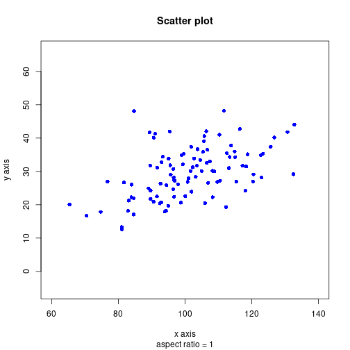
Setting parameters with par()
Formatting details of a diagram can also be controlled with a call to par() before a diagram is opened. Some aspects can be set both with par(), and with the diagram function - e.g., with options to plot(). These include (see ?par for explanations):
cex,cex.axis,cex.main,cex.labfor the size of plot symbols, axis labels and diagram titlecolfor the color of plot symbolsfont,familyfor the font of the diagram annotationslasfor the orientation of axis labelslend,lty,lwd,pchfor the style of lines and plot symbolsxaxs,yaxsfor the precise axis limitsxaxt,yaxtfor the presence of axes
Other aspects can only be set in par(). These include: bt, mar, oma, xlog, ylog. The return value of par() is a list with the old value for the changed option. When it is saved, it can later be passed as an option to par() to reset the option for the current graphics device to its previous value.
par(mfrow=c(1, 2))
op <- par(col="gray60", family="serif", bty="n", mar=c(7, 5, 7, 1), pch=16)
plot(rnorm(10), main="Changed formatting")
par(op)
plot(rnorm(10), main="Standard format")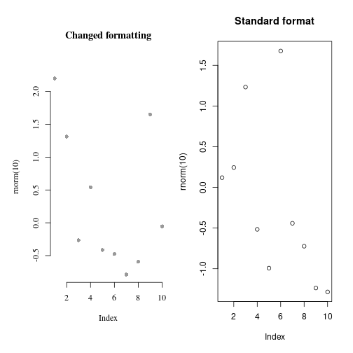
Colors
Default palette and other palette choices
N <- 6
(colDef <- palette()[1:N])
[1] "black" "red" "green3" "blue" "cyan" "magenta"(colAll <- sample(colors(), N, replace=FALSE))[1] "gray33" "khaki2" "mistyrose1" "darkslategray1"
[5] "royalblue4" "mediumorchid" colRain <- rainbow(N)
colTopo <- topo.colors(N)
colCm <- cm.colors(N)
colHeat <- heat.colors(N)len <- 1/N
xLeft <- rep(seq(0, 1-len, by=len), times=N)
yBot <- rep(seq(0, 1-len, by=len), each=N)
xRight <- rep(seq(len, 1, by=len), times=N)
yTop <- rep(seq(len, 1, by=len), each=N)
par(mar=c(0, 4, 1, 0) + 0.1)
plot(c(0, 1), c(0, 1), axes=FALSE, xlab=NA, ylab=NA, type="n",
asp=1, main="Colors")
rect(xLeft, yBot, xRight, yTop, border=NA,
col=c(colDef, colAll, colRain, colTopo, colCm, colHeat))
par(xpd=NA)
text(-0.05, seq(0, 1-len, length.out=N) + len/2, adj=1,
labels=c("default", "sample", "rainbow", "topo", "cm", "heat"))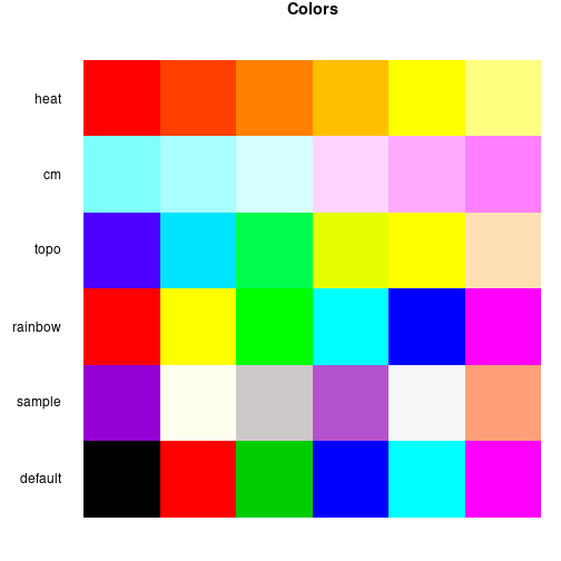
RGB colors and transparency
rgb(0, 1, 1)[1] "#00FFFF"rgb(t(col2rgb("red")/255))[1] "#FF0000"rgb(1, 0, 0, 0.5)[1] "#FF000080"N <- 150
xx <- rnorm(N, 100, 15)
yy <- 0.4*xx + rnorm(N, 0, 10)
plot(xx, yy, pch=16, cex=3.5, col=rgb(0, 0, 1, 0.3))
points(xx-20, yy-20, pch=16, cex=3.5, col=rgb(1, 0, 0, 0.3))
points(xx+20, yy-20, pch=16, cex=3.5, col=rgb(0, 1, 0, 0.3))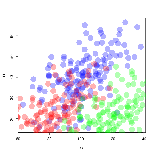
Other color spaces
hsv(0.1666, 1, 1)[1] "#FFFF00"rgb2hsv(matrix(c(0, 1, 1), nrow=3)) [,1]
h 0.500000000
s 1.000000000
v 0.003921569hcl(h=120, c=35, l=85)[1] "#BBDEB1"gray(0.5)[1] "#808080"Color palettes with RColorBrewer
N <- 6
library(RColorBrewer)
(bPal <- brewer.pal(N, "Blues"))
[1] "#EFF3FF" "#C6DBEF" "#9ECAE1" "#6BAED6" "#3182BD" "#08519C"colorRampPalette(bPal)(15) [1] "#EFF3FF" "#E0EAF9" "#D1E1F3" "#C3D9EE" "#B4D3E9" "#A6CDE4" "#96C6DF"
[8] "#84BCDB" "#72B2D7" "#5EA4D0" "#4994C7" "#3585BE" "#2574B3" "#1662A7"
[15] "#08519C"b1 <- colorRampPalette(brewer.pal(N, "Reds"))(N)
b2 <- colorRampPalette(brewer.pal(N, "Greens"))(N)
b3 <- colorRampPalette(brewer.pal(N, "BuGn"))(N)
b4 <- colorRampPalette(brewer.pal(N, "BrBG"))(N)
b5 <- colorRampPalette(brewer.pal(N, "OrRd"))(N)
b6 <- colorRampPalette(brewer.pal(N, "Accent"))(N)
len <- 1/N
xLeft <- rep(seq(0, 1-len, by=len), times=N)
yBot <- rep(seq(0, 1-len, by=len), each=N)
xRight <- rep(seq(len, 1, by=len), times=N)
yTop <- rep(seq(len, 1, by=len), each=N)
par(mar=c(0, 4, 1, 0) + 0.1)
plot(c(0, 1), c(0, 1), axes=FALSE, xlab=NA, ylab=NA, type="n",
asp=1, main="Colors")
rect(xLeft, yBot, xRight, yTop, border=NA,
col=c(b1, b2, b3, b4, b5, b6))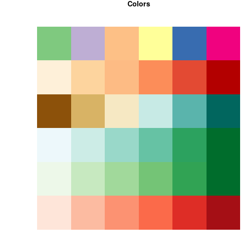
Useful packages
Package colorspace provides more functions for converting between different color spaces. The R color chart gives a very nice overview of colors available in R.
Detach (automatically) loaded packages (if possible)
try(detach(package:RColorBrewer))Get the article source from GitHub
R markdown - markdown - R code - all posts