Exploratory factor analysis for ordinal categorical data
Install required packages
GPArotation, mvtnorm, polycor, psych
wants <- c("GPArotation", "mvtnorm", "polycor", "psych")
has   <- wants %in% rownames(installed.packages())
if(any(!has)) install.packages(wants[!has])
Factor analysis
Simulate categorical data based on continuous variables
First, let’s simulate 200 observations from 6 variables, coming from 2 orthogonal factors. I’ll take a couple of intermediate steps and start with multivariate normal continuous data that I later dichotomize. That way, we can compare Pearson correlations with polychoric correlations, and compare factor loadings from continuous data with that from dichotomous data and the true loadings.
set.seed(123)
N <- 200                       # number of observations
P <- 6                         # number of variables
Q <- 2                         # number of factors

# true P x Q loading matrix -> variable-factor correlations
Lambda <- matrix(c(0.7,-0.4, 0.8,0, -0.2,0.9, -0.3,0.4, 0.3,0.7, -0.8,0.1),
                 nrow=P, ncol=Q, byrow=TRUE)
Now simulate the actual data from the model \(x = \Lambda f + e\), with \(x\) being the observed variable values of a person, \(\Lambda\) the true loadings matrix, \(f\) the latent factor score, and \(e\) iid, mean 0, normal errors.
# factor scores (uncorrelated factors)
library(mvtnorm)               # for rmvnorm()
FF <- rmvnorm(N, mean=c(5, 15), sigma=diag(Q))

# matrix with iid, mean 0, normal errors
E   <- rmvnorm(N, rep(0, P), diag(P))
X   <- FF %*% t(Lambda) + E    # matrix with variable values
dfX <- data.frame(X)           # data also as a data frame
Now let’s categorize the data. We’ll keep the data in two formats: as a data frame with ordered factors, and as a numeric matrix. hetcor() from package polycor gives us the polychoric correlation matrix we’ll later use for the FA.
# categorize variables into a list of ordered factors
lOrd <- lapply(dfX, function(x) {
               cut(x, breaks=quantile(x), include.lowest=TRUE,
                   ordered=TRUE, labels=LETTERS[1:4]) })
dfOrd  <- data.frame(lOrd)     # combine list into a data frame
ordNum <- data.matrix(dfOrd)   # categorized data as a numeric matrix
Factor analysis for ordered categorical data
Use the polychoric correlation matrix to do a regular FA.
library(polycor)               # for hetcor()
pc <- hetcor(dfOrd, ML=TRUE) # polychoric corr matrixlibrary(psych)
faPC <- fa(r=pc$correlations, nfactors=2, n.obs=N, rotate="varimax")
faPC$loadings
Loadings:
   MR2    MR1
X1  0.546 -0.196
X2  0.607
X3 -0.173  0.842
X4 -0.197  0.311
X5  0.336  0.537
X6 -0.619

                 MR2   MR1
SS loadings    1.231 1.133
Proportion Var 0.205 0.189
Cumulative Var 0.205 0.394
It is possible to skip the step of calculating the polychoric correlation matrix, and directly use fa.poly() from package psych, which does the same thing in the end. This function accepts the raw dichotomous data as a numeric matrix.
# polychoric FA
faPCdirect <- fa.poly(ordNum, nfactors=2, rotate="varimax")faPCdirect$fa$loadings # loadings are the same as above ...
Loadings:
   MR2    MR1
X1  0.546 -0.196
X2  0.605
X3 -0.174  0.841
X4 -0.198  0.311
X5  0.336  0.538
X6 -0.621

                 MR2   MR1
SS loadings    1.231 1.133
Proportion Var 0.205 0.189
Cumulative Var 0.205 0.394
Factor scores
For factor scores, look at package ltm which has a factor.scores() function specifically for polytomous outcome data. An example is provided on this page -> “Factor Scores - Ability Estimates”.
Visualize loadings
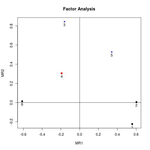
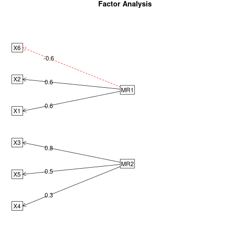
You can visualize the loadings from the factor analysis using factor.plot() and fa.diagram(), both from package psych. For some reason, factor.plot() accepts only the $fa component of the result from fa.poly(), not the full object.
factor.plot(faPCdirect$fa, cut=0.5)
fa.diagram(faPCdirect)
Determine number of factors
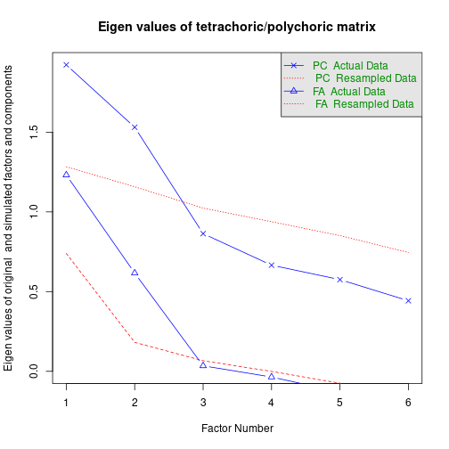
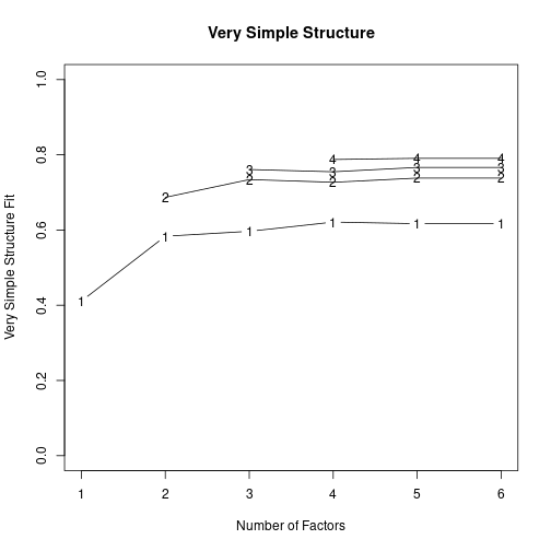
Parallel analysis and a “very simple structure” analysis provide help in selecting the number of factors. Again, package psych has the required functions. vss() takes the polychoric correlation matrix as an argument.
fap <- fa.parallel.poly(ordNum) # parallel analysis for dichotomous data
fapCall: fa.parallel.poly(x = ordNum)
Parallel analysis suggests that the number of factors = 1 and the number of components = 1
Eigen Values of
Original factors Simulated data Original components simulated data NA
1 1.23 1 10 0.79 0.28
NA NA NA NA NA NA NA NA NA NA NA NA NA NA NA
1 0.94 0.81 0.15 0.38 1.05 0.67 -0.37 -1.9 0.09 1.92 1 10 1.27 0.08 1.25
NA NA NA NA NA NA NA NA
1 1.26 0.08 1.18 1.39 0.21 0.38 -1.66 0.03vss(pc$correlations, n.obs=N, rotate="varimax") # very simple structure
Very Simple Structure
Call: vss(x = pc$correlations, rotate = "varimax", n.obs = N)
VSS complexity 1 achieves a maximimum of 0.61  with  6  factors
VSS complexity 2 achieves a maximimum of 0.76  with  6  factors

The Velicer MAP achieves a minimum of NA  with  1  factors
BIC achieves a minimum of  NA  with  2  factors
Sample Size adjusted BIC achieves a minimum of  NA  with  2  factors

Statistics by number of factors
  vss1 vss2   map dof   chisq    prob sqresid  fit RMSEA BIC SABIC complex
1 0.41 0.00 0.076   9 7.8e+01 4.9e-13    4.56 0.41 0.198  30 58.38     1.0
2 0.58 0.69 0.107   4 7.9e+00 9.4e-02    2.43 0.69 0.072 -13 -0.59     1.3
3 0.60 0.73 0.223   0 4.4e-01      NA    1.85 0.76    NA  NA    NA     1.4
4 0.60 0.69 0.400  -3 0.0e+00      NA    1.67 0.78    NA  NA    NA     1.6
5 0.56 0.75 1.000  -5 1.7e-13      NA    1.31 0.83    NA  NA    NA     1.5
6 0.61 0.76    NA  -6 0.0e+00      NA    0.85 0.89    NA  NA    NA     1.4
   eChisq    SRMR eCRMS eBIC
1 1.3e+02 1.5e-01 0.188   80
2 7.1e+00 3.4e-02 0.066  -14
3 3.6e-01 7.7e-03    NA   NA
4 8.2e-15 1.2e-09    NA   NA
5 1.5e-13 5.1e-09    NA   NA
6 3.3e-26 2.4e-15    NA   NA
Detach (automatically) loaded packages (if possible)
try(detach(package:GPArotation))
try(detach(package:psych))
try(detach(package:polycor))
try(detach(package:sfsmisc))
try(detach(package:mvtnorm))
(based on an answer I wrote on CrossValidated)
Get the article source from GitHub
R markdown - markdown - R code - all posts