Nonparametric bootstrapping

TODO

• link to resamplingBootALM

Install required packages

boot

wants <- c("boot")
has   <- wants %in% rownames(installed.packages())
if(any(!has)) install.packages(wants[!has])

Confidence interval for \(\mu\)

Using package boot

set.seed(123)
muH0 <- 100
sdH0 <- 40
N    <- 200
DV   <- rnorm(N, muH0, sdH0)

Function to calculate the mean and uncorrected variance (=plug-in estimator for the population variance) of a given replication.

getM <- function(orgDV, idx) {
    n     <- length(orgDV[idx])
    bsM   <- mean(orgDV[idx])
    bsS2M <- (((n-1) / n) * var(orgDV[idx])) / n
    c(bsM, bsS2M)
}

library(boot)
nR     <- 999
(bsRes <- boot(DV, statistic=getM, R=nR))

ORDINARY NONPARAMETRIC BOOTSTRAP


Call:
boot(data = DV, statistic = getM, R = nR)


Bootstrap Statistics :
     original      bias    std. error
t1* 99.657182 0.068458482   2.6470886
t2*  7.080822 0.001496239   0.7552599

Various types of bootstrap confidence intervals

alpha <- 0.05
boot.ci(bsRes, conf=1-alpha, type=c("basic", "perc", "norm", "stud", "bca"))

BOOTSTRAP CONFIDENCE INTERVAL CALCULATIONS
Based on 999 bootstrap replicates

CALL : 
boot.ci(boot.out = bsRes, conf = 1 - alpha, type = c("basic", 
    "perc", "norm", "stud", "bca"))

Intervals : 
Level      Normal              Basic             Studentized     
95%   ( 94.40, 104.78 )   ( 94.51, 104.70 )   ( 94.58, 104.76 )  

Level     Percentile            BCa          
95%   ( 94.62, 104.80 )   ( 94.39, 104.67 )  
Calculations and Intervals on Original Scale

Bootstrap distribution

For the \(t\) test statistic, compare the empirical distribution from the bootstrap replicates against the theoretical \(t_{n-1}\) distribtion.

res    <- replicate(nR, getM(DV, sample(seq(along=DV), replace=TRUE)))
Mstar  <- res[1, ]
SMstar <- sqrt(res[2, ])
tStar  <- (Mstar-mean(DV)) / SMstar

plot(tStar, ecdf(tStar)(tStar), col="gray60", pch=1, xlab="t* bzw. t",
     ylab="P(T <= t)", main="t*: cumulative rel. frequency and t CDF")
curve(pt(x, N-1), lwd=2, add=TRUE)
legend(x="topleft", lty=c(NA, 1), pch=c(1, NA), lwd=c(2, 2),
       col=c("gray60", "black"), legend=c("t*", "t"))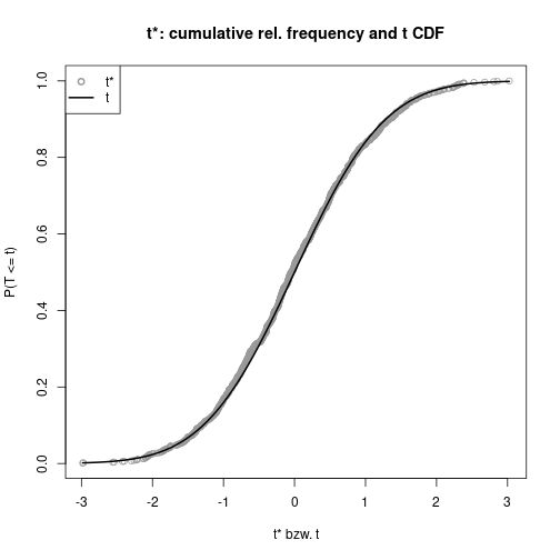

Detailed information about bootstrap samples

boot.array(boot(...), indices=TRUE) gives detailed information about the selected indices for each bootstrap replication. If the sample has \(n\) observations, and there are \(R\) replications, the result is an \((R \times n)\)-matrix with one row for each replication and one column for each observation.

bootIdx <- boot.array(bsRes, indices=TRUE)

# replications 1-3: first 10 selected indices in each replication
bootIdx[1:3, 1:10]

     [,1] [,2] [,3] [,4] [,5] [,6] [,7] [,8] [,9] [,10]
[1,]  111   76  119   87   28  142   25  140   51    19
[2,]   23   19  144  106  178   59   70  187    9    76
[3,]  195   52   93   66   93  153   23  116   44   182

# selected indices in the first replication
repl1Idx <- bootIdx[1, ]

# selected values in the first replication
repl1DV <- DV[repl1Idx]
head(repl1DV, n=5) 

[1]  76.98612 141.02285  66.01183 143.87356 106.13492

Detach (automatically) loaded packages (if possible)

try(detach(package:boot))

Get the article source from GitHub

R markdown - markdown - R code - all posts