One-way ANOVA (CR-p design)
TODO
- link to normality, varianceHom, regressionDiag, regression for model comparison, resamplingPerm, resamplingBootALM
Install required packages
wants <- c("car", "DescTools", "multcomp")
has   <- wants %in% rownames(installed.packages())
if(any(!has)) install.packages(wants[!has])CR-\(p\) ANOVA
Simulate data
set.seed(123)
P     <- 4
Nj    <- c(41, 37, 42, 40)
muJ   <- rep(c(-1, 0, 1, 2), Nj)
dfCRp <- data.frame(IV=factor(rep(LETTERS[1:P], Nj)),
DV=rnorm(sum(Nj), muJ, 5))plot.design(DV ~ IV, fun=mean, data=dfCRp, main="Group means")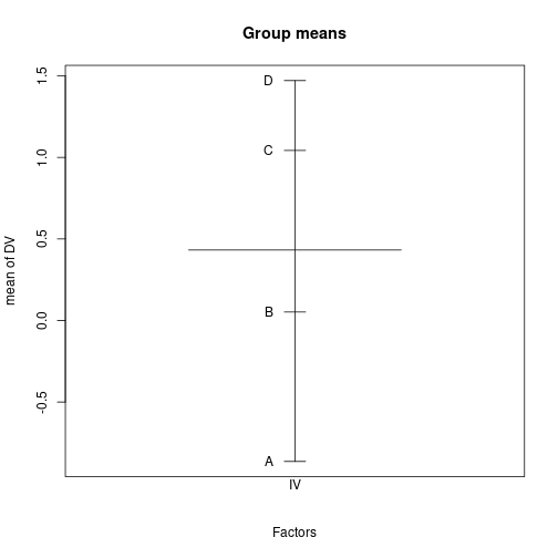
Using oneway.test()
Assuming variance homogeneity
oneway.test(DV ~ IV, data=dfCRp, var.equal=TRUE)
    One-way analysis of means

data:  DV and IV
F = 2.0057, num df = 3, denom df = 156, p-value = 0.1154
Generalized Welch-test without assumption of variance homogeneity
oneway.test(DV ~ IV, data=dfCRp, var.equal=FALSE)
    One-way analysis of means (not assuming equal variances)

data:  DV and IV
F = 2.0203, num df = 3.000, denom df = 85.503, p-value = 0.1171
Using aov()
aovCRp <- aov(DV ~ IV, data=dfCRp)
summary(aovCRp)
Df Sum Sq Mean Sq F value Pr(>F)
IV 3 133 44.35 2.006 0.115
Residuals 156 3450 22.11 model.tables(aovCRp, type="means")Tables of means
Grand mean
0.4318522
IV
A B C D
-0.8643 0.05185 1.042 1.471
rep 41.0000 37.00000 42.000 40.000Model comparisons using anova(lm())
(anovaCRp <- anova(lm(DV ~ IV, data=dfCRp)))Analysis of Variance Table
Response: DV
Df Sum Sq Mean Sq F value Pr(>F)
IV 3 133.1 44.353 2.0057 0.1154
Residuals 156 3449.7 22.113 anova(lm(DV ~ 1, data=dfCRp), lm(DV ~ IV, data=dfCRp))Analysis of Variance Table
Model 1: DV ~ 1
Model 2: DV ~ IV
Res.Df RSS Df Sum of Sq F Pr(>F)
1 159 3582.8
2 156 3449.7 3 133.06 2.0057 0.1154anovaCRp["Residuals", "Sum Sq"][1] 3449.703Effect size estimates
dfSSb <- anovaCRp["IV",        "Df"]
SSb   <- anovaCRp["IV",        "Sum Sq"]
MSb   <- anovaCRp["IV",        "Mean Sq"]
SSw   <- anovaCRp["Residuals", "Sum Sq"]
MSw   <- anovaCRp["Residuals", "Mean Sq"]
\(\hat{\eta^{2}}\)
(etaSq <- SSb / (SSb + SSw))[1] 0.03713889library(DescTools) # for EtaSq()
EtaSq(aovCRp, type=1)Error in EtaSq.lm(aovCRp, type = 1): konnte Funktion "is" nicht finden\(\hat{\omega^{2}}\), \(\hat{f^{2}}\)
(omegaSq <- dfSSb * (MSb-MSw) / (SSb + SSw + MSw))[1] 0.01850809(f <- sqrt(etaSq / (1-etaSq)))[1] 0.196396Planned comparisons - a-priori
General contrasts using glht() from package multcomp
cntrMat <- rbind("A-D"          =c(  1,   0,   0,  -1),
                 "1/3*(A+B+C)-D"=c(1/3, 1/3, 1/3,  -1),
                 "B-C"          =c(  0,   1,  -1,   0))
library(multcomp)                      # for glht()
summary(glht(aovCRp, linfct=mcp(IV=cntrMat), alternative="less"),
        test=adjusted("none"))
     Simultaneous Tests for General Linear Hypotheses

Multiple Comparisons of Means: User-defined Contrasts


Fit: aov(formula = DV ~ IV, data = dfCRp)

Linear Hypotheses:
                   Estimate Std. Error t value Pr(<t)
A-D >= 0            -2.3351     1.0451  -2.234 0.0134 *
1/3*(A+B+C)-D >= 0  -1.3941     0.8589  -1.623 0.0533 .
B-C >= 0            -0.9906     1.0603  -0.934 0.1758
---
Signif. codes:  0 '***' 0.001 '**' 0.01 '*' 0.05 '.' 0.1 ' ' 1
(Adjusted p values reported -- none method)
Pairwise \(t\)-tests
pairwise.t.test(dfCRp$DV, dfCRp$IV, p.adjust.method="bonferroni")
    Pairwise comparisons using t tests with pooled SD

data:  dfCRp$DV and dfCRp$IV

  A    B    C
B 1.00 -    -
C 0.40 1.00 -
D 0.16 1.00 1.00

P value adjustment method: bonferroni
Planned comparisons - post-hoc
Scheffe tests
library(DescTools)                  # for ScheffeTest()
ScheffeTest(aovCRp, which="IV", contrasts=t(cntrMat))
  Posthoc multiple comparisons of means : Scheffe Test
    95% family-wise confidence level

$IV
              diff    lwr.ci    upr.ci   pval
A-D     -2.3351002 -5.288758 0.6185575 0.1770
A,B,C-D -1.3941211 -3.821531 1.0332885 0.4538
B-C     -0.9906183 -3.987210 2.0059738 0.8319

---
Signif. codes: 0 `***' 0.001 `**' 0.01 `*' 0.05 `.' 0.1 ` ' 1
Tukey’s simultaneous confidence intervals
(tHSD <- TukeyHSD(aovCRp)) Tukey multiple comparisons of means
95% family-wise confidence level
Fit: aov(formula = DV ~ IV, data = dfCRp)
$IV
diff lwr upr p adj
B-A 0.9161596 -1.8529795 3.685299 0.8257939
C-A 1.9067779 -0.7743204 4.587876 0.2555117
D-A 2.3351002 -0.3789061 5.049107 0.1185540
C-B 0.9906183 -1.7628388 3.744075 0.7864641
D-B 1.4189406 -1.3665697 4.204451 0.5497967
D-C 0.4283223 -2.2696814 3.126326 0.9762890plot(tHSD)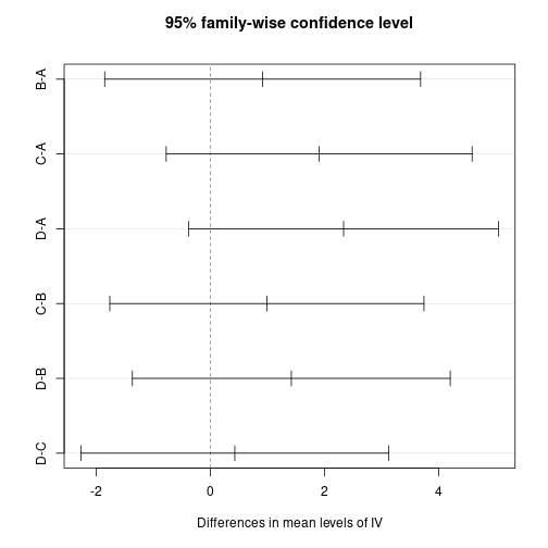
Using glht() from package multcomp
library(multcomp)                      # for glht()
tukey <- glht(aovCRp, linfct=mcp(IV="Tukey"))
summary(tukey)
     Simultaneous Tests for General Linear Hypotheses

Multiple Comparisons of Means: Tukey Contrasts


Fit: aov(formula = DV ~ IV, data = dfCRp)

Linear Hypotheses:
           Estimate Std. Error t value Pr(>|t|)
B - A == 0   0.9162     1.0663   0.859    0.826
C - A == 0   1.9068     1.0324   1.847    0.255
D - A == 0   2.3351     1.0451   2.234    0.119
C - B == 0   0.9906     1.0603   0.934    0.786
D - B == 0   1.4189     1.0726   1.323    0.550
D - C == 0   0.4283     1.0389   0.412    0.976
(Adjusted p values reported -- single-step method)confint(tukey)
     Simultaneous Confidence Intervals

Multiple Comparisons of Means: Tukey Contrasts


Fit: aov(formula = DV ~ IV, data = dfCRp)

Quantile = 2.5972
95% family-wise confidence level


Linear Hypotheses:
           Estimate lwr     upr
B - A == 0  0.9162  -1.8533  3.6856
C - A == 0  1.9068  -0.7746  4.5882
D - A == 0  2.3351  -0.3792  5.0494
C - B == 0  0.9906  -1.7632  3.7444
D - B == 0  1.4189  -1.3669  4.2048
D - C == 0  0.4283  -2.2700  3.1266
Assess test assumptions
Normality
Estud <- rstudent(aovCRp)
qqnorm(Estud, pch=20, cex=2)
qqline(Estud, col="gray60", lwd=2)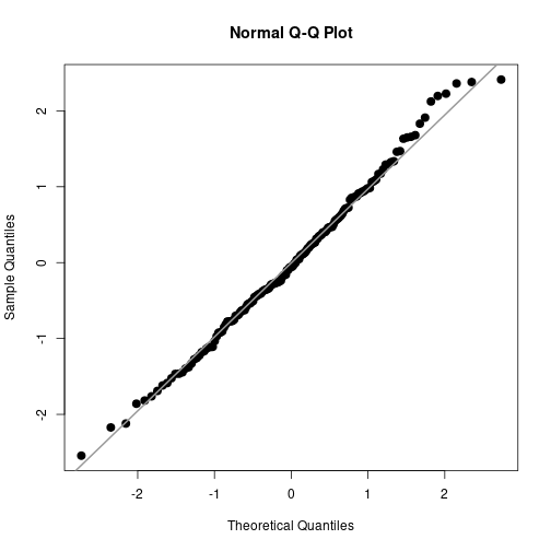
shapiro.test(Estud)
    Shapiro-Wilk normality test

data:  Estud
W = 0.9937, p-value = 0.7149
Variance homogeneity
plot(Estud ~ dfCRp$IV, main="Residuals per group")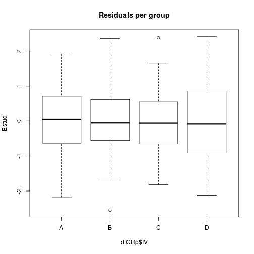
library(car)
leveneTest(aovCRp)
Levene's Test for Homogeneity of Variance (center = median)
Df F value Pr(>F)
group 3 0.8551 0.4659
156 Detach (automatically) loaded packages (if possible)
try(detach(package:car))
try(detach(package:multcomp))
try(detach(package:survival))
try(detach(package:mvtnorm))
try(detach(package:splines))
try(detach(package:TH.data))
try(detach(package:DescTools))
Get the article source from GitHub
R markdown - markdown - R code - all posts