Frequency tables
Install required packages
wants <- c("DescTools")
has   <- wants %in% rownames(installed.packages())
if(any(!has)) install.packages(wants[!has])
Category frequencies for one variable
Absolute frequencies
set.seed(123)
(myLetters <- sample(LETTERS[1:5], 12, replace=TRUE))
[1] "B" "D" "C" "E" "E" "A" "C" "E" "C" "C" "E" "C"(tab <- table(myLetters))myLetters
A B C D E
1 1 5 1 4 names(tab)[1] "A" "B" "C" "D" "E"tab["B"]B
1 barplot(tab, main="Counts")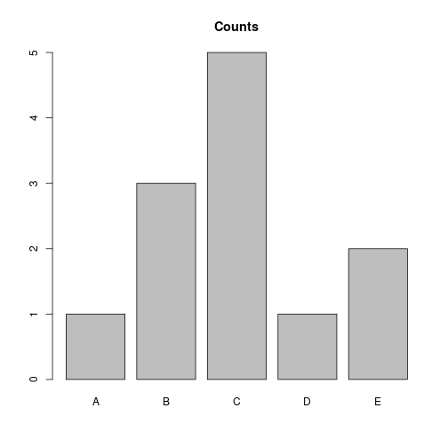
(Cumulative) relative frequencies
(relFreq <- prop.table(tab))myLetters
A B C D E
0.08333333 0.08333333 0.41666667 0.08333333 0.33333333 cumsum(relFreq) A B C D E
0.08333333 0.16666667 0.58333333 0.66666667 1.00000000 Counting non-existent categories
letFac <- factor(myLetters, levels=c(LETTERS[1:5], "Q"))
letFac
[1] B D C E E A C E C C E C
Levels: A B C D E Qtable(letFac)letFac
A B C D E Q
1 1 5 1 4 0 Counting runs
(vec <- rep(rep(c("f", "m"), 3), c(1, 3, 2, 4, 1, 2))) [1] "f" "m" "m" "m" "f" "f" "m" "m" "m" "m" "f" "m" "m"(res <- rle(vec))Run Length Encoding
lengths: int [1:6] 1 3 2 4 1 2
values : chr [1:6] "f" "m" "f" "m" "f" "m"length(res$lengths)[1] 6inverse.rle(res) [1] "f" "m" "m" "m" "f" "f" "m" "m" "m" "m" "f" "m" "m"Contingency tables for two or more variables
Absolute frequencies using table()
N    <- 10
(sex <- factor(sample(c("f", "m"), N, replace=TRUE)))
[1] m m f m f f f m m m
Levels: f m(work <- factor(sample(c("home", "office"), N, replace=TRUE))) [1] office office office office office office home home office office
Levels: home office(cTab <- table(sex, work)) work
sex home office
f 1 3
m 1 5summary(cTab)Number of cases in table: 10
Number of factors: 2
Test for independence of all factors:
Chisq = 0.10417, df = 1, p-value = 0.7469
Chi-squared approximation may be incorrectbarplot(cTab, beside=TRUE, legend.text=rownames(cTab), ylab="absolute frequency")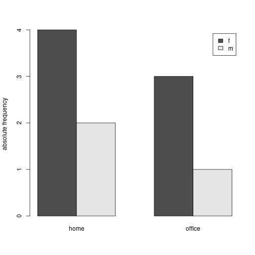
Using xtabs()
counts   <- sample(0:5, N, replace=TRUE)
(persons <- data.frame(sex, work, counts))
sex work counts
1 m office 4
2 m office 4
3 f office 0
4 m office 2
5 f office 4
6 f office 1
7 f home 1
8 m home 1
9 m office 0
10 m office 2xtabs(~ sex + work, data=persons) work
sex home office
f 1 3
m 1 5xtabs(counts ~ sex + work, data=persons) work
sex home office
f 1 5
m 1 12Marginal sums and means
apply(cTab, MARGIN=1, FUN=sum)f m
4 6 colMeans(cTab) home office
1 4 addmargins(cTab, c(1, 2), FUN=mean)Margins computed over dimensions
in the following order:
1: sex
2: work work
sex home office mean
f 1.0 3.0 2.0
m 1.0 5.0 3.0
mean 1.0 4.0 2.5Relative frequencies
(relFreq <- prop.table(cTab)) work
sex home office
f 0.1 0.3
m 0.1 0.5Conditional relative frequencies
prop.table(cTab, margin=1) work
sex home office
f 0.2500000 0.7500000
m 0.1666667 0.8333333prop.table(cTab, margin=2) work
sex home office
f 0.500 0.375
m 0.500 0.625Flat contingency tables for more than two variables
(group <- factor(sample(c("A", "B"), 10, replace=TRUE))) [1] A A A A A A A B A A
Levels: A Bftable(work, sex, group, row.vars="work", col.vars=c("sex", "group")) sex f m
group A B A B
work
home 1 0 0 1
office 3 0 5 0Recovering the original data from contingency tables
Individual-level data frame
library(DescTools)
Untable(cTab)
sex work
1 f home
2 m home
3 f office
4 f office
5 f office
6 m office
7 m office
8 m office
9 m office
10 m officeGroup-level data frame
as.data.frame(cTab, stringsAsFactors=TRUE) sex work Freq
1 f home 1
2 m home 1
3 f office 3
4 m office 5Percentile rank
(vec <- round(rnorm(10), 2)) [1] 0.84 0.15 -1.14 1.25 0.43 -0.30 0.90 0.88 0.82 0.69Fn <- ecdf(vec)
Fn(vec) [1] 0.7 0.3 0.1 1.0 0.4 0.2 0.9 0.8 0.6 0.5100 * Fn(0.1)[1] 20Fn(sort(vec)) [1] 0.1 0.2 0.3 0.4 0.5 0.6 0.7 0.8 0.9 1.0knots(Fn) [1] -1.14 -0.30 0.15 0.43 0.69 0.82 0.84 0.88 0.90 1.25plot(Fn, main="cumulative frequencies")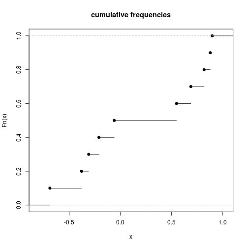
Detach (automatically) loaded packages (if possible)
try(detach(package:DescTools))Get the article source from GitHub
R markdown - markdown - R code - all posts