Two-way ANOVA (CRF-pq design)
TODO
- link to anovaSStypes, normality, varianceHom, regressionDiag
- use
model.tables()
Install required packages
car, DescTools, multcomp, phia
wants <- c("car", "DescTools", "multcomp", "phia")
has   <- wants %in% rownames(installed.packages())
if(any(!has)) install.packages(wants[!has])CRF-\(pq\) ANOVA
Using aov() (SS type I)
set.seed(123)
Njk  <- 8
P    <- 2
Q    <- 3
muJK <- c(rep(c(1, -1), Njk), rep(c(2, 1), Njk), rep(c(3, 3), Njk))
dfCRFpq <- data.frame(IV1=factor(rep(1:P, times=Njk*Q)),
                      IV2=factor(rep(1:Q,  each=Njk*P)),
DV =rnorm(Njk*P*Q, muJK, 2))dfCRFpq$IVcomb <- interaction(dfCRFpq$IV1, dfCRFpq$IV2)aovCRFpq <- aov(DV ~ IV1*IV2, data=dfCRFpq)
summary(aovCRFpq) Df Sum Sq Mean Sq F value Pr(>F)
IV1 1 15.75 15.75 4.371 0.042644 *
IV2 2 73.95 36.98 10.259 0.000236 ***
IV1:IV2 2 10.62 5.31 1.474 0.240669
Residuals 42 151.38 3.60
---
Signif. codes: 0 '***' 0.001 '**' 0.01 '*' 0.05 '.' 0.1 ' ' 1Using Anova() from package car (SS type II or III)
Since this design has equal cell sizes, all SS types give the same result.
# change contrasts for SS type III
fitIII <- lm(DV ~ IV1 + IV2 + IV1:IV2, data=dfCRFpq,
             contrasts=list(IV1=contr.sum, IV2=contr.sum))
library(car)                           # for Anova()
Anova(fitIII, type="III")
Anova Table (Type III tests)
Response: DV
Sum Sq Df F value Pr(>F)
(Intercept) 114.229 1 31.6922 1.352e-06 ***
IV1 15.755 1 4.3711 0.0426439 *
IV2 73.951 2 10.2587 0.0002356 ***
IV1:IV2 10.624 2 1.4737 0.2406692
Residuals 151.381 42
---
Signif. codes: 0 '***' 0.001 '**' 0.01 '*' 0.05 '.' 0.1 ' ' 1Plot marginal and cell means
plot.design(DV ~ IV1*IV2, data=dfCRFpq, main="Marginal means")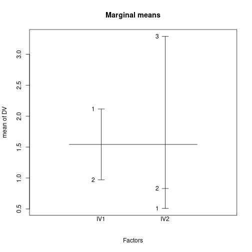
interaction.plot(dfCRFpq$IV1, dfCRFpq$IV2, dfCRFpq$DV,
                 main="Cell means", col=c("red", "blue", "green"), lwd=2)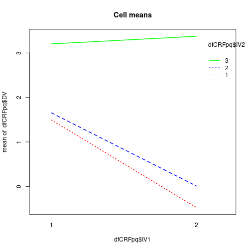
Effect size estimate: partial \(\hat{\eta}_{p}^{2}\)
library(DescTools)
EtaSq(aovCRFpq, type=1)
Error in EtaSq.lm(aovCRFpq, type = 1): konnte Funktion "is" nicht findenSimple effects
library(phia)
testInteractions(aovCRFpq, fixed="IV2", across="IV1", adjustment="none")
F Test:
P-value adjustment method: none
Value Df Sum of Sq F Pr(>F)
1 1.96713 1 15.478 4.2944 0.04441 *
2 1.64183 1 10.782 2.9915 0.09105 .
3 -0.17151 1 0.118 0.0326 0.85749
Residuals 42 151.381
---
Signif. codes: 0 '***' 0.001 '**' 0.01 '*' 0.05 '.' 0.1 ' ' 1testInteractions(aovCRFpq, fixed="IV1", across="IV2", adjustment="none")F Test:
P-value adjustment method: none
IV21 IV22 Df Sum of Sq F Pr(>F)
1 -1.7098 -1.5508 2 14.276 1.9804 0.1506926
2 -3.8484 -3.3641 2 70.299 9.7520 0.0003321 ***
Residuals 42 151.381
---
Signif. codes: 0 '***' 0.001 '**' 0.01 '*' 0.05 '.' 0.1 ' ' 1Planned comparisons
Main effects only
Free comparisons of marginal means
cMat <- rbind("c1"=c( 1/2, 1/2, -1),
              "c2"=c(  -1,   0,  1))

library(multcomp)
summary(glht(aovCRFpq, linfct=mcp(IV2=cMat), alternative="two.sided"),
        test=adjusted("bonferroni"))
     Simultaneous Tests for General Linear Hypotheses

Multiple Comparisons of Means: User-defined Contrasts


Fit: aov(formula = DV ~ IV1 * IV2, data = dfCRFpq)

Linear Hypotheses:
        Estimate Std. Error t value Pr(>|t|)
c1 == 0  -1.6303     0.8221  -1.983    0.108
c2 == 0   1.7098     0.9493   1.801    0.158
(Adjusted p values reported -- bonferroni method)
Tukey simultaneous confidence intervals
Fit model without interaction that is ignored by Tukey’s HSD.
aovCRF <- aov(DV ~ IV1 + IV2, data=dfCRFpq)
TukeyHSD(aovCRF, which="IV2")
Tukey multiple comparisons of means
95% family-wise confidence level
Fit: aov(formula = DV ~ IV1 + IV2, data = dfCRFpq)
$IV2
diff lwr upr p adj
2-1 0.3216154 -1.3238577 1.967089 0.8838220
3-1 2.7790779 1.1336047 4.424551 0.0005109
3-2 2.4574624 0.8119893 4.102936 0.0021302Using glht() from package multcomp.
library(multcomp)
tukey <- glht(aovCRF, linfct=mcp(IV2="Tukey"))
summary(tukey)
     Simultaneous Tests for General Linear Hypotheses

Multiple Comparisons of Means: Tukey Contrasts


Fit: aov(formula = DV ~ IV1 + IV2, data = dfCRFpq)

Linear Hypotheses:
           Estimate Std. Error t value Pr(>|t|)
2 - 1 == 0   0.3216     0.6784   0.474 0.883804
3 - 1 == 0   2.7791     0.6784   4.096 0.000521 ***
3 - 2 == 0   2.4575     0.6784   3.622 0.002147 **
---
Signif. codes:  0 '***' 0.001 '**' 0.01 '*' 0.05 '.' 0.1 ' ' 1
(Adjusted p values reported -- single-step method)confint(tukey)
     Simultaneous Confidence Intervals

Multiple Comparisons of Means: Tukey Contrasts


Fit: aov(formula = DV ~ IV1 + IV2, data = dfCRFpq)

Quantile = 2.4264
95% family-wise confidence level


Linear Hypotheses:
           Estimate lwr     upr
2 - 1 == 0  0.3216  -1.3245  1.9677
3 - 1 == 0  2.7791   1.1330  4.4252
3 - 2 == 0  2.4575   0.8114  4.1035
Cell comparisons using the associated one-way ANOVA
(aovCRFpqA <- aov(DV ~ IVcomb, data=dfCRFpq))Call:
aov(formula = DV ~ IVcomb, data = dfCRFpq)
Terms:
IVcomb Residuals
Sum of Squares 100.3295 151.3812
Deg. of Freedom 5 42
Residual standard error: 1.898503
Estimated effects may be unbalancedcntrMat <- rbind("c1"=c(-1/2, 1/4, -1/2, 1/4, 1/4, 1/4),
"c2"=c( 0, 0, -1, 0, 1, 0),
"c3"=c(-1/2, -1/2, 1/4, 1/4, 1/4, 1/4))library(multcomp)
summary(glht(aovCRFpqA, linfct=mcp(IVcomb=cntrMat), alternative="greater"),
test=adjusted("none"))
     Simultaneous Tests for General Linear Hypotheses

Multiple Comparisons of Means: User-defined Contrasts


Fit: aov(formula = DV ~ IVcomb, data = dfCRFpq)

Linear Hypotheses:
        Estimate Std. Error t value  Pr(>t)
c1 <= 0 -0.04422    0.58130  -0.076 0.53014
c2 <= 0  1.55080    0.94925   1.634 0.05490 .
c3 <= 0  1.55035    0.58130   2.667 0.00541 **
---
Signif. codes:  0 '***' 0.001 '**' 0.01 '*' 0.05 '.' 0.1 ' ' 1
(Adjusted p values reported -- none method)
Post-hoc Scheffe tests using the associated one-way ANOVA
library(DescTools)
ScheffeTest(aovCRFpqA, which="IVcomb", contrasts=t(cntrMat))
  Posthoc multiple comparisons of means : Scheffe Test
    95% family-wise confidence level

$IVcomb
                               diff     lwr.ci   upr.ci   pval
2.1,2.2,1.3,2.3-1.1,1.2 -0.04422288 -2.0736407 1.985195 1.0000
1.3-1.2                  1.55079557 -1.7632298 4.864821 0.7494
1.2,2.2,1.3,2.3-1.1,2.1  1.55034667 -0.4790711 3.579764 0.2360

---
Signif. codes: 0 `***' 0.001 `**' 0.01 `*' 0.05 `.' 0.1 ` ' 1
Post-hoc Scheffe tests for marginal means
library(DescTools)
ScheffeTest(aovCRFpq, which="IV2", contrasts=c(-1, 1/2, 1/2))
  Posthoc multiple comparisons of means : Scheffe Test
    95% family-wise confidence level

$IV2
          diff     lwr.ci   upr.ci   pval
2,3-1 1.550347 -0.4790711 3.579764 0.2360

---
Signif. codes: 0 `***' 0.001 `**' 0.01 `*' 0.05 `.' 0.1 ` ' 1
Assess test assumptions
Normality
Estud <- rstudent(aovCRFpq)
qqnorm(Estud, pch=20, cex=2)
qqline(Estud, col="gray60", lwd=2)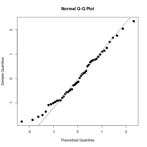
shapiro.test(Estud)
    Shapiro-Wilk normality test

data:  Estud
W = 0.9771, p-value = 0.4655
Variance homogeneity
plot(Estud ~ dfCRFpq$IVcomb, main="Residuals per group")
library(car)
leveneTest(aovCRFpq)
Levene's Test for Homogeneity of Variance (center = median)
Df F value Pr(>F)
group 5 0.048 0.9985
42 Detach (automatically) loaded packages (if possible)
try(detach(package:phia))
try(detach(package:car))
try(detach(package:multcomp))
try(detach(package:survival))
try(detach(package:mvtnorm))
try(detach(package:splines))
try(detach(package:TH.data))
try(detach(package:DescTools))
Get the article source from GitHub
R markdown - markdown - R code - all posts