Association tests and measures for ordered categorical variables

TODO
Install required packages
Linear-by-linear association test
Polychoric and polyserial correlation
Association measures involving categorical and continuous variables
- AUC, Kendall’s \(\tau_{a}\), Somers’ \(D_{xy}\), Goodman & Kruskal’s \(\gamma\)
- Area under the ROC-curve (AUC)
Detach (automatically) loaded packages (if possible)
Get the article source from GitHub

TODO

link to correlation, association, diagCategorical

Install required packages

coin, mvtnorm, polycor, pROC, rms

wants <- c("coin", "mvtnorm", "polycor", "pROC", "rms")
has   <- wants %in% rownames(installed.packages())
if(any(!has)) install.packages(wants[!has])

Linear-by-linear association test

set.seed(123)
library(mvtnorm)
N     <- 100
Sigma <- matrix(c(4,2,-3, 2,16,-1, -3,-1,9), byrow=TRUE, ncol=3)
mu    <- c(-3, 2, 4)
Xdf   <- data.frame(rmvnorm(n=N, mean=mu, sigma=Sigma))

lOrd   <- lapply(Xdf, function(x) {
                 cut(x, breaks=quantile(x), include.lowest=TRUE,
                     ordered=TRUE, labels=LETTERS[1:4]) })
dfOrd  <- data.frame(lOrd)
matOrd <- data.matrix(dfOrd)

cTab <- xtabs(~ X1 + X3, data=dfOrd)
addmargins(cTab)

     X3
X1      A   B   C   D Sum
  A     1   5   6  13  25
  B     5   7   6   7  25
  C     8   9   4   4  25
  D    11   4   9   1  25
  Sum  25  25  25  25 100

library(coin)
lbl_test(cTab, distribution=approximate(nresample=9999))


    Approximative Linear-by-Linear Association Test

data:  X3 (ordered) by X1 (A < B < C < D)
Z = -4.1391, p-value < 1e-04
alternative hypothesis: two.sided

Polychoric and polyserial correlation

Polychoric correlation

library(polycor)
polychor(dfOrd$X1, dfOrd$X2, ML=TRUE)

[1] 0.308646

polychor(cTab, ML=TRUE)

[1] -0.4818203

Polyserial correlation

library(polycor)
polyserial(Xdf$X2, dfOrd$X3)

[1] -0.1302779

Heterogeneous correlation matrices

library(polycor)
Xdf2   <- rmvnorm(n=N, mean=mu, sigma=Sigma)
dfBoth <- cbind(Xdf2, dfOrd)
hetcor(dfBoth, ML=TRUE)


Maximum-Likelihood Estimates

Correlations/Type of Correlation:
           1        2         3         X1         X2         X3
1          1  Pearson   Pearson Polyserial Polyserial Polyserial
2     0.2792        1   Pearson Polyserial Polyserial Polyserial
3    -0.3899 -0.07191         1 Polyserial Polyserial Polyserial
X1  -0.05105  -0.1335  -0.07871          1 Polychoric Polychoric
X2   -0.1755  -0.2621   0.04899     0.3086          1 Polychoric
X3 -0.005707 -0.03443 -0.006209    -0.4818   -0.08556          1

Standard Errors:
         1       2      3      X1     X2
1                                       
2  0.09257                              
3  0.08522 0.09977                      
X1  0.1069  0.1044 0.1077               
X2  0.1033  0.1001 0.1082  0.1062       
X3  0.1071  0.1082 0.1088 0.09226 0.1132

n = 100 

P-values for Tests of Bivariate Normality:
        1      2      3     X1      X2
1                                     
2  0.8156                             
3  0.6836  0.488                      
X1  0.107 0.5607 0.5548               
X2    0.2 0.7338 0.2466 0.4721        
X3 0.4423 0.9903 0.7281 0.3579 0.04774

Association measures involving categorical and continuous variables

AUC, Kendall’s \(\tau_{a}\), Somers’ \(D_{xy}\), Goodman & Kruskal’s \(\gamma\)

One continuous variable and one dichotomous variable

N   <- 100
x   <- rnorm(N)
y   <- x + rnorm(N, 0, 2)
yDi <- ifelse(y <= median(y), 0, 1)

Nagelkerke’s pseudo-\(R^{2}\) (R2), area under the ROC-Kurve (C), Somers’ \(D_{xy}\) (Dxy), Goodman & Kruskal’s \(\gamma\) (Gamma), Kendall’s \(\tau\) (Tau-a)

library(rms)
lrm(yDi ~ x)$stats

         Obs    Max Deriv   Model L.R.         d.f.            P            C 
1.000000e+02 4.370579e-07 5.974581e+00 1.000000e+00 1.451353e-02 6.342000e-01 
         Dxy        Gamma        Tau-a           R2        Brier            g 
2.684000e-01 2.685074e-01 1.355556e-01 7.732807e-02 2.356851e-01 5.793523e-01 
          gr           gp 
1.784882e+00 1.379571e-01

Area under the ROC-curve (AUC)

library(pROC)
(rocRes <- roc(yDi ~ x, plot=TRUE, ci=TRUE, main="ROC-curve",
               xlab="specificity (TN / (TN+FP))", ylab="sensitivity (TP / (TP+FN))"))


Call:
roc.formula(formula = yDi ~ x, plot = TRUE, ci = TRUE, main = "ROC-curve",     xlab = "specificity (TN / (TN+FP))", ylab = "sensitivity (TP / (TP+FN))")

Data: x in 50 controls (yDi 0) < 50 cases (yDi 1).
Area under the curve: 0.634
95% CI: 0.5249-0.7431 (DeLong)

rocCI <- ci.se(rocRes)
plot(rocCI, type="shape")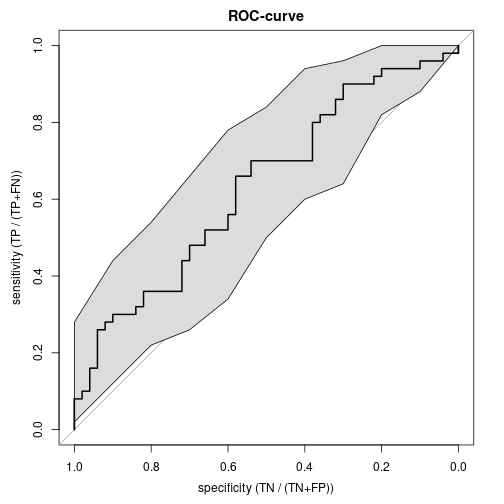

Detach (automatically) loaded packages (if possible)

try(detach(package:coin))
try(detach(package:rms))
try(detach(package:Hmisc))
try(detach(package:lattice))
try(detach(package:Formula))
try(detach(package:survival))
try(detach(package:ggplot2))
try(detach(package:pROC))
try(detach(package:polycor))
try(detach(package:mvtnorm))

Get the article source from GitHub

R markdown - markdown - R code - all posts