Diagrams for categorical data
Install required packages
wants <- c("plotrix")
has   <- wants %in% rownames(installed.packages())
if(any(!has)) install.packages(wants[!has])
Barplots
Simulate data
set.seed(123)
dice  <- sample(1:6, 100, replace=TRUE)
(dTab <- table(dice))
dice
1 2 3 4 5 6
17 16 20 14 18 15 Simple barplot
barplot(dTab, ylim=c(0, 30), xlab="Result", ylab="N", col="black",
        main="Absolute frequency")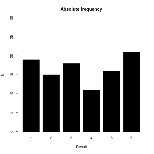
barplot(prop.table(dTab), ylim=c(0, 0.3), xlab="Result",
        ylab="relative frequency", col="gray50",
        main="Relative frequency")
# not shown
Barplots for contingency tables of two variables
Stacked barplot
roll1   <- dice[1:50]
roll2   <- dice[51:100]
rollAll <- rbind(table(roll1), table(roll2))
rownames(rollAll) <- c("first", "second"); rollAll
1 2 3 4 5 6
first 8 9 8 7 7 11
second 9 7 12 7 11 4barplot(rollAll, beside=FALSE, legend.text=TRUE, xlab="Result", ylab="N",
main="Absolute frequency in two samples")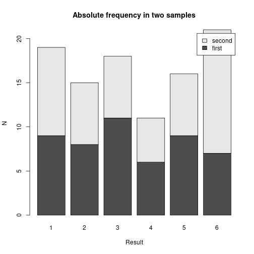
Grouped barplot
barplot(rollAll, beside=TRUE, ylim=c(0, 15), col=c("red", "green"),
        legend.text=TRUE, xlab="Result", ylab="N",
        main="Absolute frequency in two samples")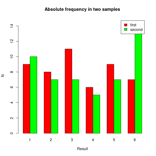
Spineplot
N      <- 100
age    <- sample(18:45, N, replace=TRUE)
drinks <- c("beer", "red wine", "white wine")
pref   <- factor(sample(drinks, N, replace=TRUE))
xRange <- round(range(age), -1) + c(-10, 10)
lims   <- c(18, 25, 35, 45)
spineplot(x=age, y=pref, xlab="Age class", ylab="drink", breaks=lims,
          main="Preferred drink by age class")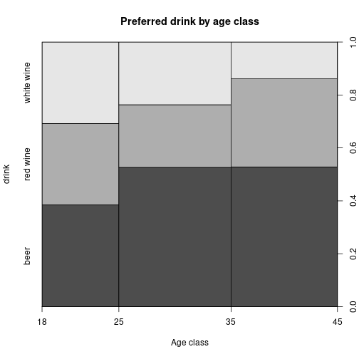
Mosaic-plot
ageCls <- cut(age, breaks=lims, labels=LETTERS[1:(length(lims)-1)])
group  <- factor(sample(letters[1:2], N, replace=TRUE))
cTab   <- table(ageCls, pref, group)
mosaicplot(cTab, cex.axis=1)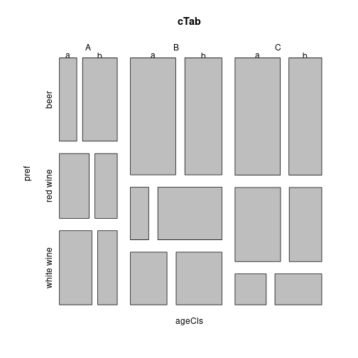
Pie-charts
2-D pie-chart
dice <- sample(1:6, 100, replace=TRUE)
dTab <- table(dice)
pie(dTab, col=c("blue", "red", "yellow", "pink", "green", "orange"),
    main="Relative frequencies from rolling dice")

dTabFreq <- prop.table(dTab)
textRad  <- 0.5
angles   <- dTabFreq * 2 * pi
csAngles <- cumsum(angles)
csAngles <- csAngles - angles/2
textX    <- textRad * cos(csAngles)
textY    <- textRad * sin(csAngles)
text(x=textX, y=textY, labels=dTabFreq)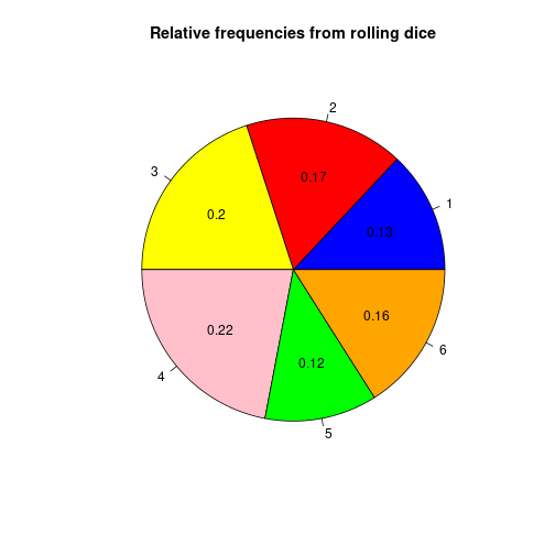
3-D pie-chart
library(plotrix)
pie3D(dTab, theta=pi/4, explode=0.1, labels=names(dTab))
Conditional density plot
N    <- 100
X    <- rnorm(N, 175, 7)
Y    <- 0.5*X + rnorm(N, 0, 6)
Yfac <- cut(Y, breaks=c(-Inf, median(Y), Inf), labels=c("lo", "hi"))
myDf <- data.frame(X, Yfac)cdplot(Yfac ~ X, data=myDf)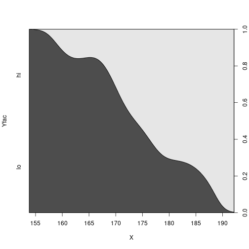
Useful packages
More plot types for categorical data are available in packages vcd and vcdExtra.
Detach (automatically) loaded packages (if possible)
try(detach(package:plotrix))Get the article source from GitHub
R markdown - markdown - R code - all posts